HFRL Unit-1
Summary
-
Reinforcement Learning is a method where an agent learns by interacting with its environment, using trial and error and feedback from rewards.
-
The goal of an RL agent is to maximize its expected cumulative reward, based on the idea that all goals can be framed as maximizing this reward.
-
The RL process is a loop that outputs a sequence of state, action, reward, and next state.
-
Expected cumulative reward is calculated by discounting future rewards, giving more weight to immediate rewards since they are more predictable than long-term ones.
-
To solve an RL problem, we find an optimal policy, the AI’s “brain” that decides the best action for each state to maximize expected return.
Two ways to find Optimal Policy
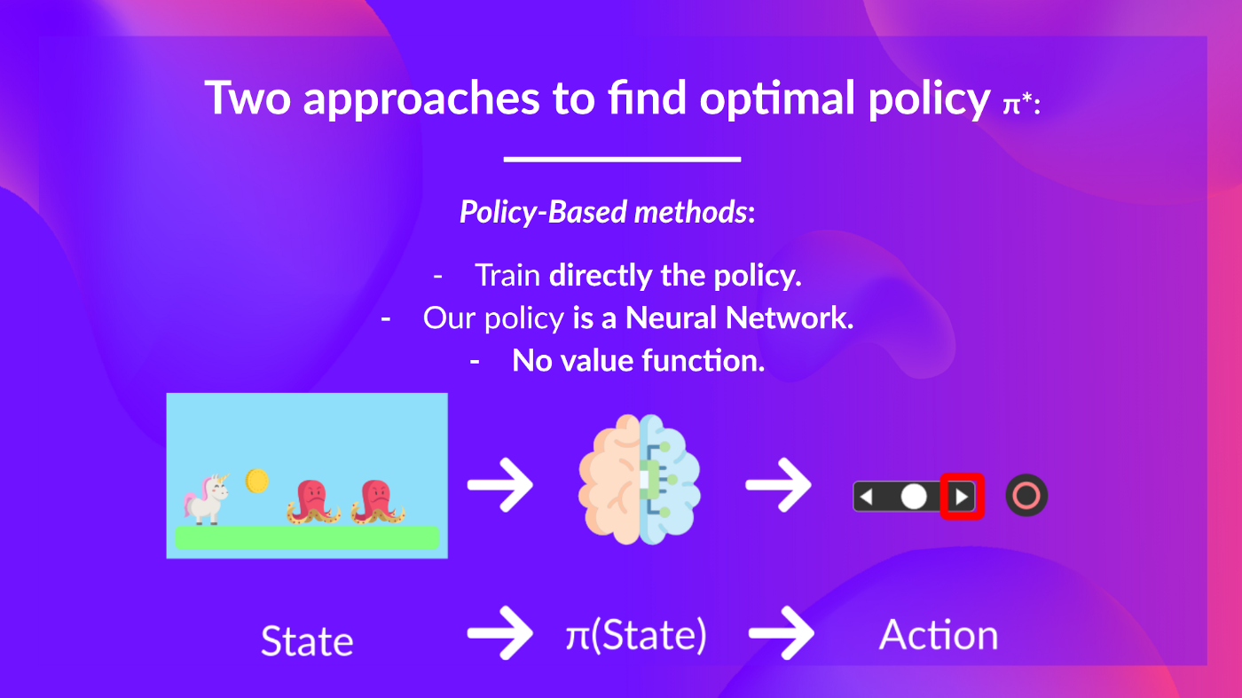
- Policy-based methods directly optimize the policy by adjusting its parameters to maximize expected return.
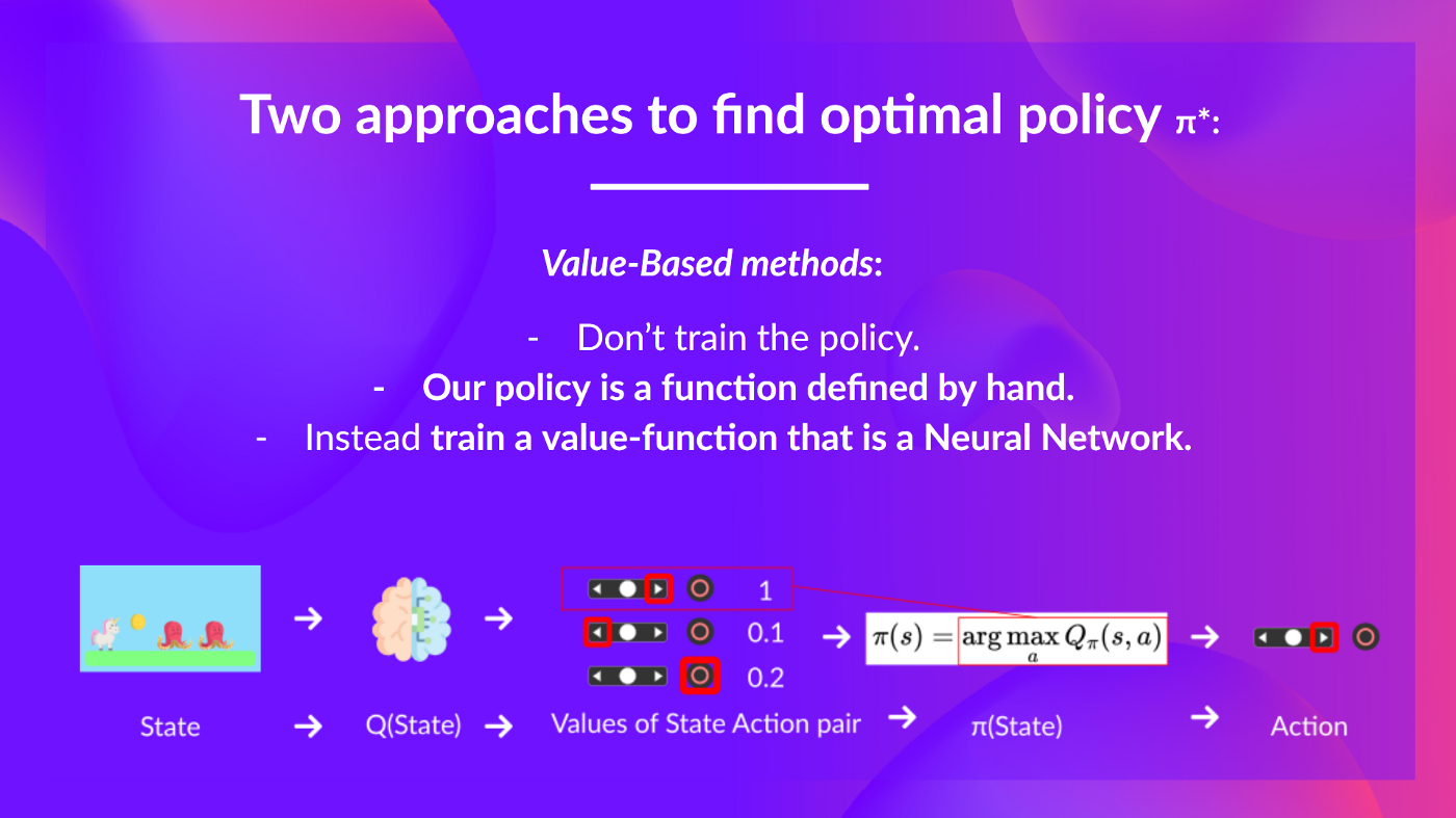
- Value-based methods train a value function that estimates the expected return for each state and use it to define the policy.
Deep RL is “Deep” because it uses deep neural networks to estimate the action to take (policy-based) or to estimate the value of a state (value-based).
HFRL Unit-2
Value-based methods
-
Value-based methods estimate the value of each state (or state-action pair) and derive the policy from these values.
-
We learn a value function that maps a state to the expected value of being at that state.

-
The value of a state is the expected discounted return obtained by following the policy from that state.
What does it mean to “follow a policy”?
- The goal of an RL agent is to have an optimal policy $\pi^*$ that maximizes the expected return from any state.
- Policy-based methods $\rightarrow$ directly train the policy to select what action to take given a state $\rightarrow \pi(a|s) \rightarrow$ We do not need to learn a value function.
- Policy takes the current state as input and outputs an action or a distribution over possible actions.
- We don’t define the policy explicitly; instead, we learn it through interactions with the environment.
- Value-based methods $\rightarrow$ trains the policy indirectly by learning a value function $\rightarrow V(s) \rightarrow$ We do not need to learn the policy explicitly.
- The value function takes the current state as input and outputs the expected return (value) of that state.
- The policy is not trained or learned directly $\rightarrow$ it is derived from the value function given specific rules.
- For example, a common rule is to select the action that leads to the state with the highest value (greedy policy).
- Policy-based methods $\rightarrow$ directly train the policy to select what action to take given a state $\rightarrow \pi(a|s) \rightarrow$ We do not need to learn a value function.
The Difference between Value-based and Policy-based methods
- In policy-based methods, the policy is learned directly by training a neural network to output actions based on states.
- Optimal policy $\pi^*$ is learned directly.
- In value-based methods, the policy is derived from a learned value function, which estimates the expected return of states.
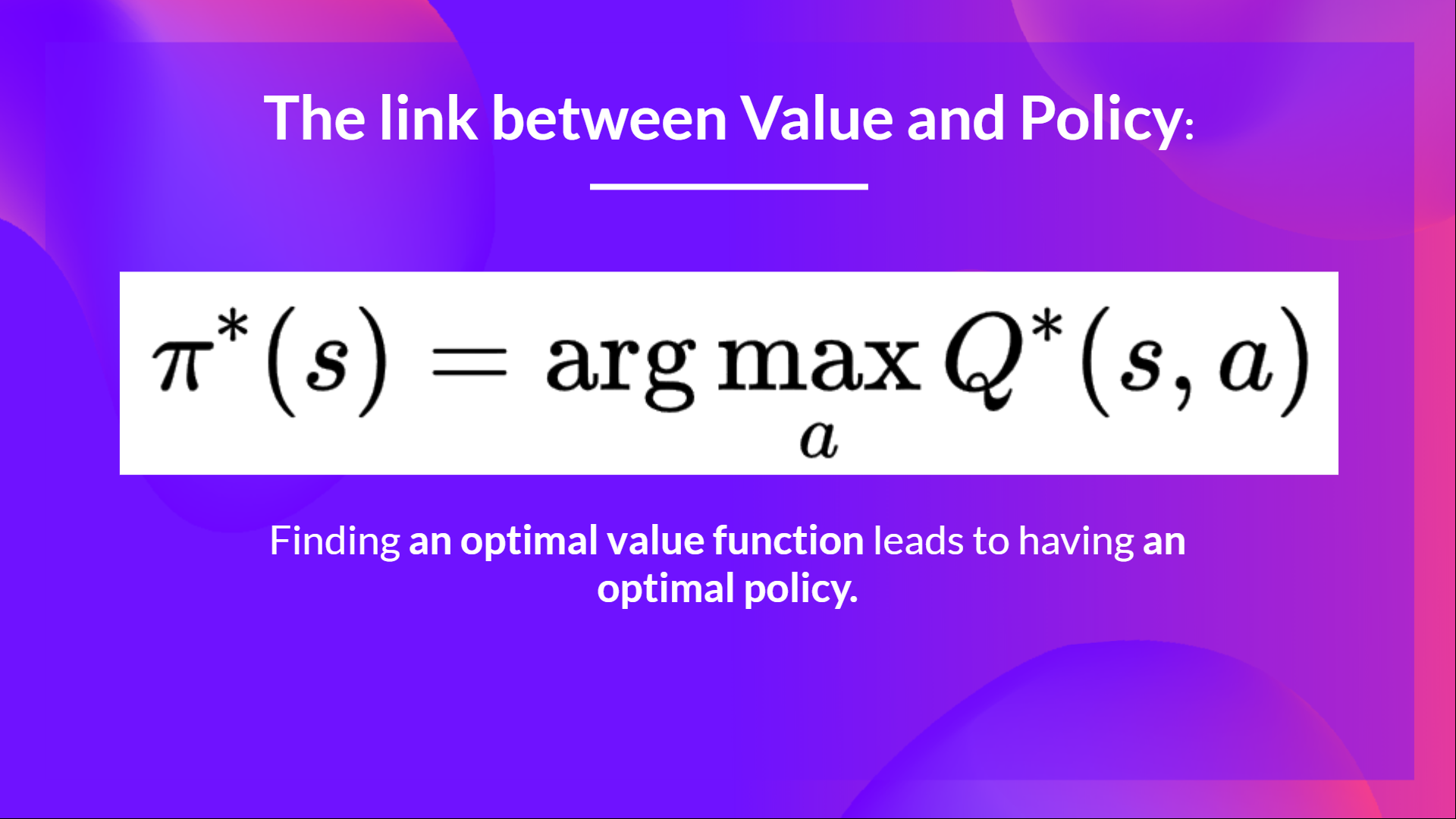
- Optimal policy $ \pi^* $ is derived from the optimal value function $ V^* $$(s)$ or the action-value function $ Q^*(s, a) $.
- Optimal policy $ \pi^* $ is derived from the optimal value function $ V^* $$(s)$ or the action-value function $ Q^*(s, a) $.
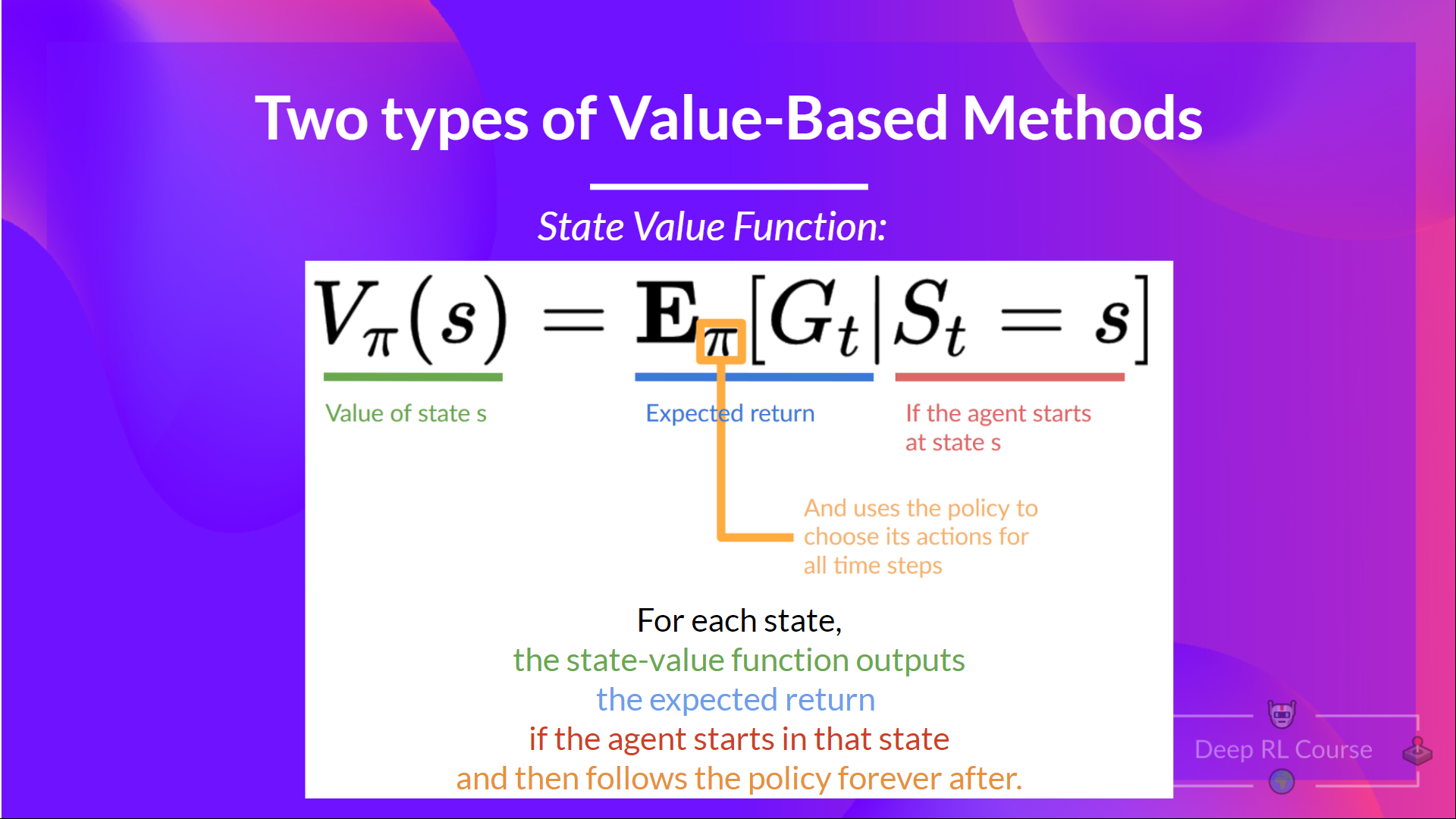
Two types of Value Functions
- State-Value Function $V_\pi(s)$: Estimates the expected return starting from state $s$ and following policy $\pi$.
- It gives the value of being in a particular state.
- Formula: $$V_\pi(s) = \mathbb{E}_\pi [G_t | S_t = s]$$
- Where $G_t$ is the return (cumulative discounted reward) from time step $t$.
- Action-Value Function $Q_\pi(s, a)$: Estimates the expected return starting from state $s$, taking action $a$, and following policy $\pi$ thereafter.
- It gives the value of taking a particular action in a particular state.
- Formula:
$$Q_\pi(s, a) = \mathbb{E}_\pi [G_t | S_t = s, A_t = a]$$

Difference: The state-value function evaluates the value of being in a state, while the action-value function evaluates the value of taking a specific action in a state.
Both case are used to derive the optimal policy $\pi^*$ by selecting actions that maximize the expected return.
Problem: To calculate the value of a state or state-action pair, we need to know the expected return $G_t$, which depends on future rewards and the policy $\pi$. This can be computationally expensive and complex, especially in environments with many states and actions. Bellman equations provide a recursive way to compute these values efficiently.
Bellman Equations
-
Simplifies the computation of value functions ($V_\pi(s)$ and $Q_\pi(s, a)$) by breaking them down into immediate rewards and the value of subsequent states.
-
Instead of calculating the expected return for each state or each state-action pair, we can use the Bellman equation.
-
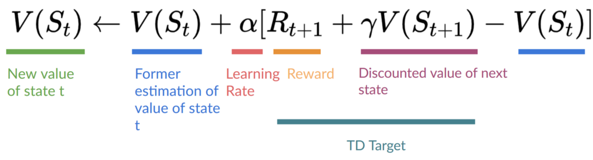
The Bellman equation expresses a state’s value recursively as the immediate reward plus the discounted value of the next state:
$$V(S_t) = R_{t+1} + \gamma V(S_{t+1})$$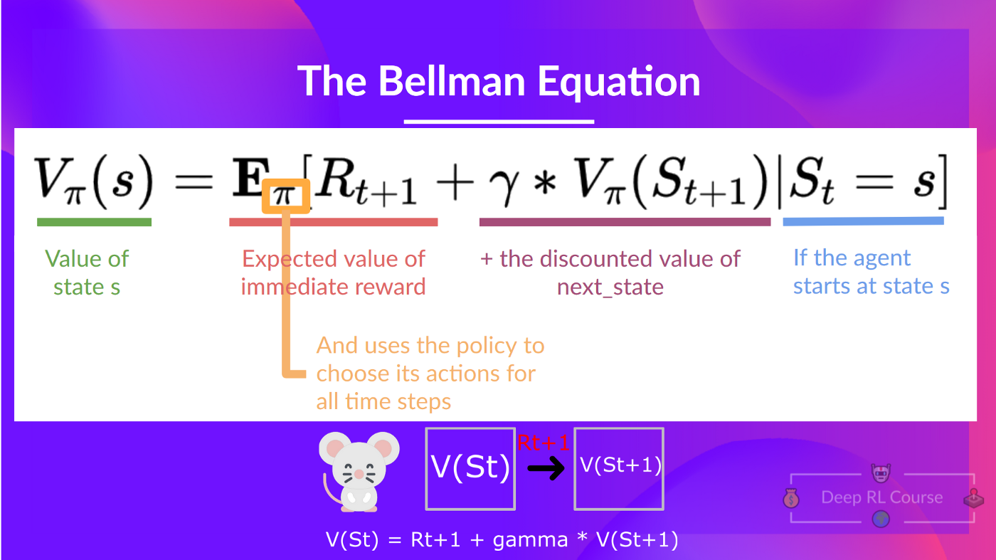
-
In summary, the Bellman equation simplifies value estimation by expressing it as the immediate reward plus the discounted value of the next state.
-
Monte Carlo methods and Temporal Difference (TD) learning are two primary approaches to estimate value functions in reinforcement learning.
Monte Carlo Methods
- Monte Carlo waits until the end of an episode to calculate the total return ($G_t$) and then updates the value function ($V_\pi(s)$ or $Q_\pi(s, a)$) based on this return.
- It requires complete episodes.
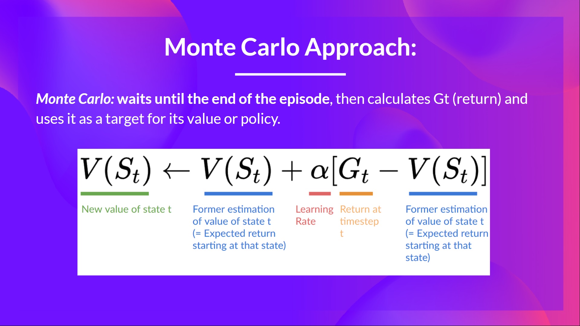
- The update rule for the state-value function is: $$V(S_t) \leftarrow V(S_t) + \alpha [G_t - V(S_t)]$$
- Where $\alpha$ is the learning rate, and $G_t$ is the total return from time step $t$.
- Then restart the episode and repeat.
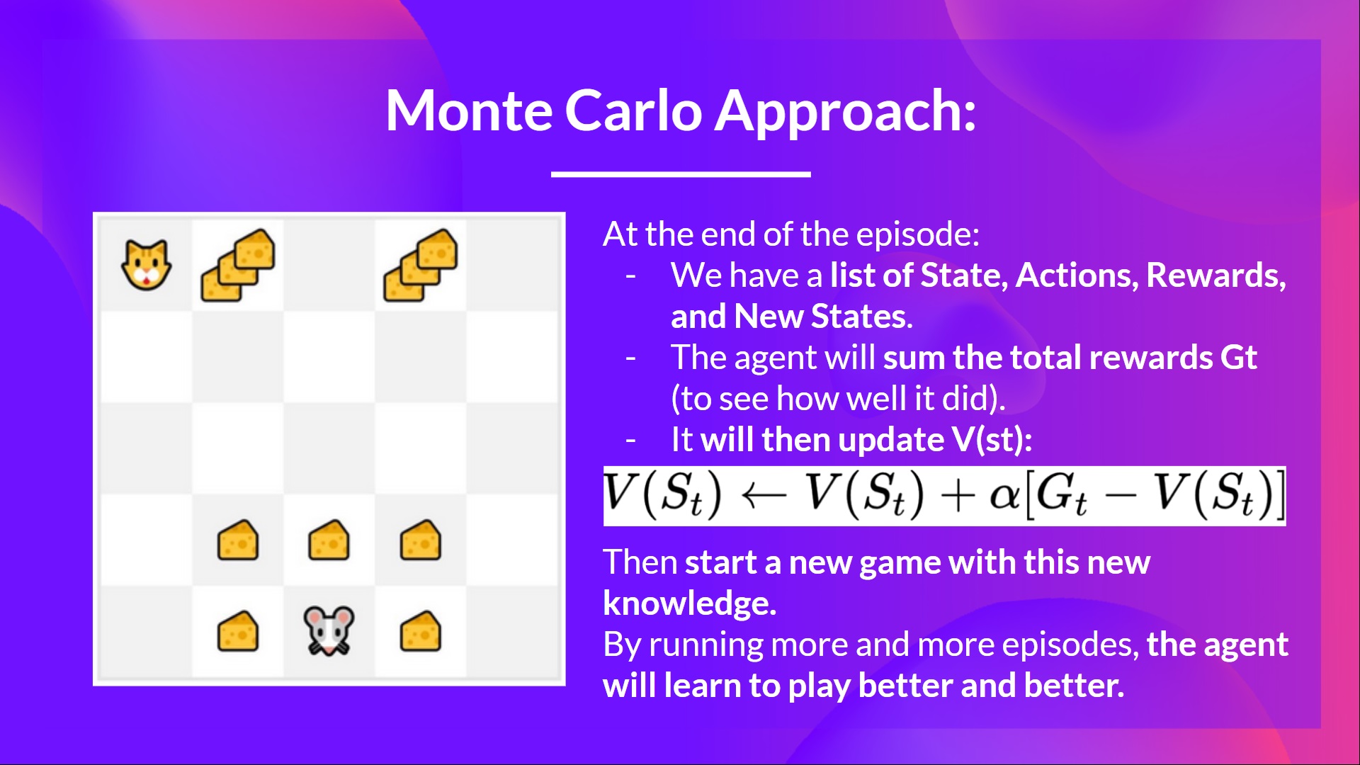
Example of Monte Carlo:
- We initialize the value function $V(s)$ arbitrarily (e.g., all zeros) for all states $s$.
- Our learning rate $\alpha$ is set to 0.1 and discount factor $\gamma$ is 1 (for simplicity).
- We run an episode in the environment, collecting states, actions, and rewards until the episode ends.
- At the end of the episode, we calculate the return $G_t$ for each time step $t$.
- We update the value function for each state visited during the episode using the update rule.
- We repeat this process for many episodes, gradually improving our value function estimates.
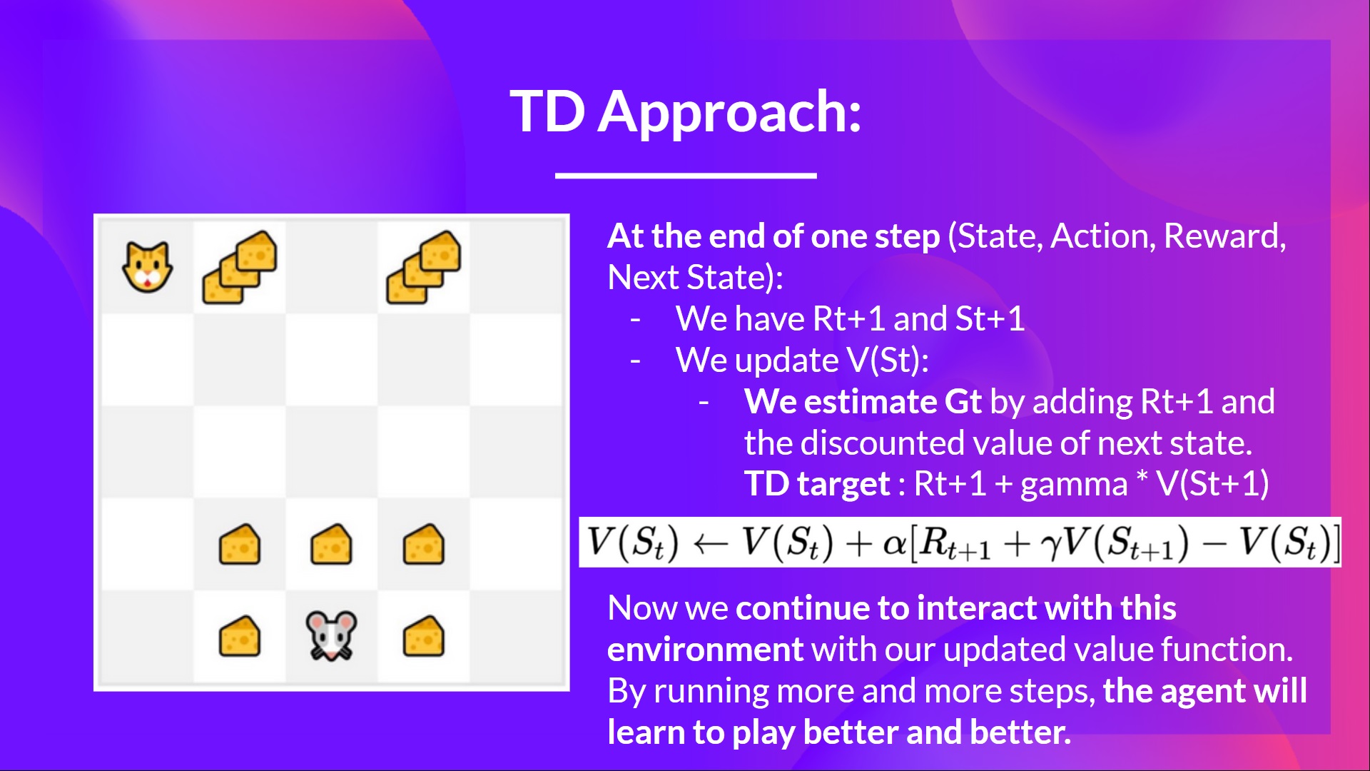
Temporal Difference (TD) Learning
- TD learning updates the value function ($V_\pi(s)$ or $Q_\pi(s, a)$) at each time step using the immediate reward and the estimated value of the next state.
- It does not require complete episodes and can learn from incomplete sequences.
- Because we didn’t wait until the end of the episode, we don’t have the full return $G_t$.
- Instead, we use the immediate reward $R_{t+1}$ and the estimated value of the next state $V(S_{t+1})$ to update our value function.
- This is called bootstrapping because we are using our current estimate to improve itself incrementally.
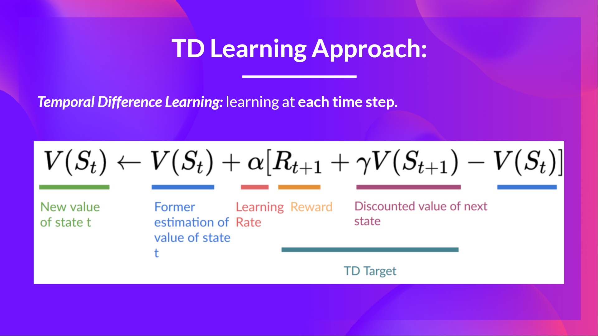
- The update rule for the state-value function is: $$V(S_t) \leftarrow V(S_t) + \alpha [R_{t+1} + \gamma V(S_{t+1}) - V(S_t)]$$
- Where $\alpha$ is the learning rate, $R_{t+1}$ is the immediate reward, and $V(S_{t+1})$ is the estimated value of the next state.
- Then move to the next state and repeat.
- This method is known as TD(0) because it updates the value function based on a one-step lookahead.
- The estimated return is known as the TD target: $$\text{TD Target} = R_{t+1} + \gamma V(S_{t+1})$$
Summary of Monte Carlo vs TD Learning
| Aspect | Monte Carlo Methods | Temporal Difference (TD) Learning |
|---|---|---|
| Update Timing | Updates value function at the end of an episode | Updates value function at each time step |
| Requirement | Requires complete episodes | Can learn from incomplete sequences |
| Return Calculation | Uses total return $G_t$ | Uses immediate reward and estimated next state value |
| Bootstrapping | No | Yes |
On-policy vs Off-policy Learning
- On-policy methods learn the value of the policy being executed (the same policy used to make decisions).
- Example: SARSA (State-Action-Reward-State-Action)
- Off-policy methods learn the value of a different policy than the one being executed (the behavior policy).
- Example: Q-learning
Q-learning
-
Q-Learning is an off-policy value-based method that uses a TD approach to train its action-value function $Q(s, a)$.
-
Approximate the optimal action-value function $Q^*(s, a)$, which gives the maximum expected return for taking action $a$ in state $s$ and following the optimal policy thereafter.

-
The value of a state, or a state-action pair is the expected cumulative reward our agent gets if it starts at this state (or state-action pair) and then acts accordingly to its policy.
-
The reward is the feedback the agent gets from the environment after taking an action.
-
Q-function is encoded in a table called Q-table:
State Action 1 Action 2 Action 3 S1 Q(S1,A1) Q(S1,A2) Q(S1,A3) S2 Q(S2,A1) Q(S2,A2) Q(S2,A3) S3 Q(S3,A1) Q(S3,A2) Q(S3,A3) -
The agent selects actions based on the Q-values in the table, typically choosing the action with the highest Q-value for the current state (greedy policy).
-
The Q-values are updated using the Q-learning update rule:
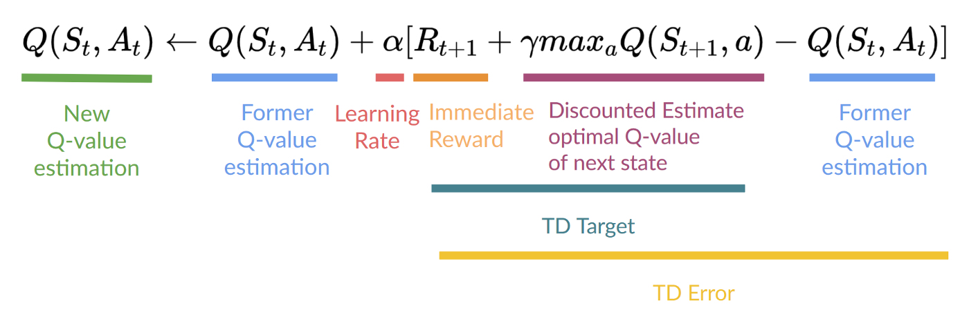
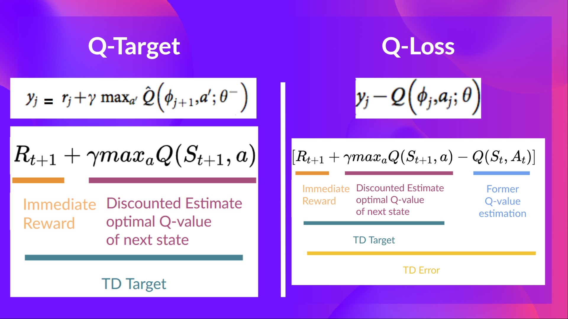
$$Q(S_t, A_t) \leftarrow Q(S_t, A_t) + \alpha [R_{t+1} + \gamma \max_a Q(S_{t+1}, a) - Q(S_t, A_t)]$$ -
Where $\alpha$ is the learning rate, $R_{t+1}$ is the immediate reward, $\gamma$ is the discount factor, and $\max_a Q(S_{t+1}, a)$ is the maximum estimated Q-value for the next state $S_{t+1}$ over all possible actions $a$.
-
The term $R_{t+1} + \gamma \max_a Q(S_{t+1}, a)$ is known as the TD target in Q-learning.
-
The agent updates the Q-value for the current state-action pair based on the immediate reward and the maximum estimated Q-value for the next state.
-
This update is done at each time step, allowing the agent to learn from each interaction with the environment.
-
Q-function returns the expected cumulative reward for taking action $a$ in state $s$ and following the optimal policy thereafter.
Summary of Q-learning
- Trains Q-function $Q(s, a)$ $\rightarrow$ action-value function $\rightarrow$ internally uses Q-table that maps state-action pairs to values.
- Given a state and an action, Q-function returns the expected cumulative reward for taking that action in that state and following the optimal policy thereafter.
- After training, the optimal policy $\pi^*$ can be derived by selecting the action with the highest Q-value for each state: $$\pi^*(s) = \arg\max_a Q^*(s, a)$$
- Q-learning is an off-policy method because it learns the optimal policy independently of the
Q-learning Algorithm
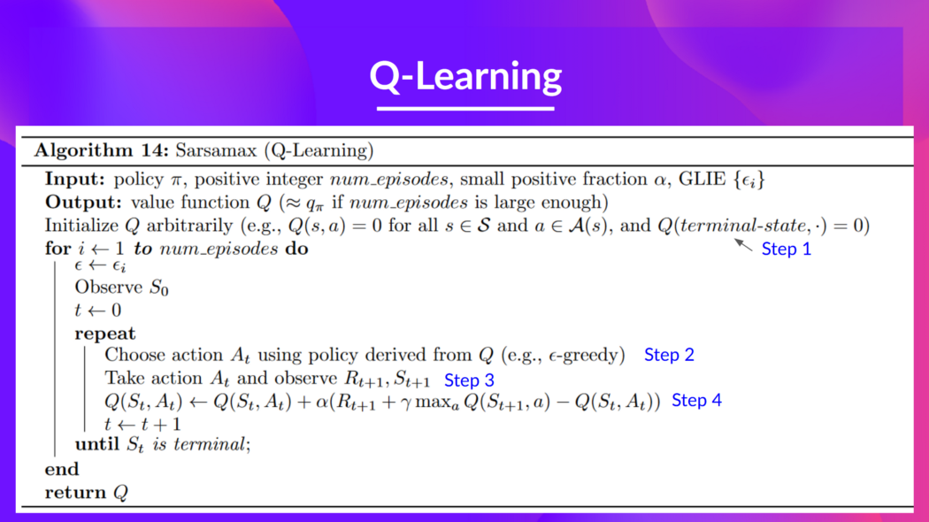
- Step 1: Initialize the Q-table with arbitrary values (e.g., all zeros) for all state-action pairs.
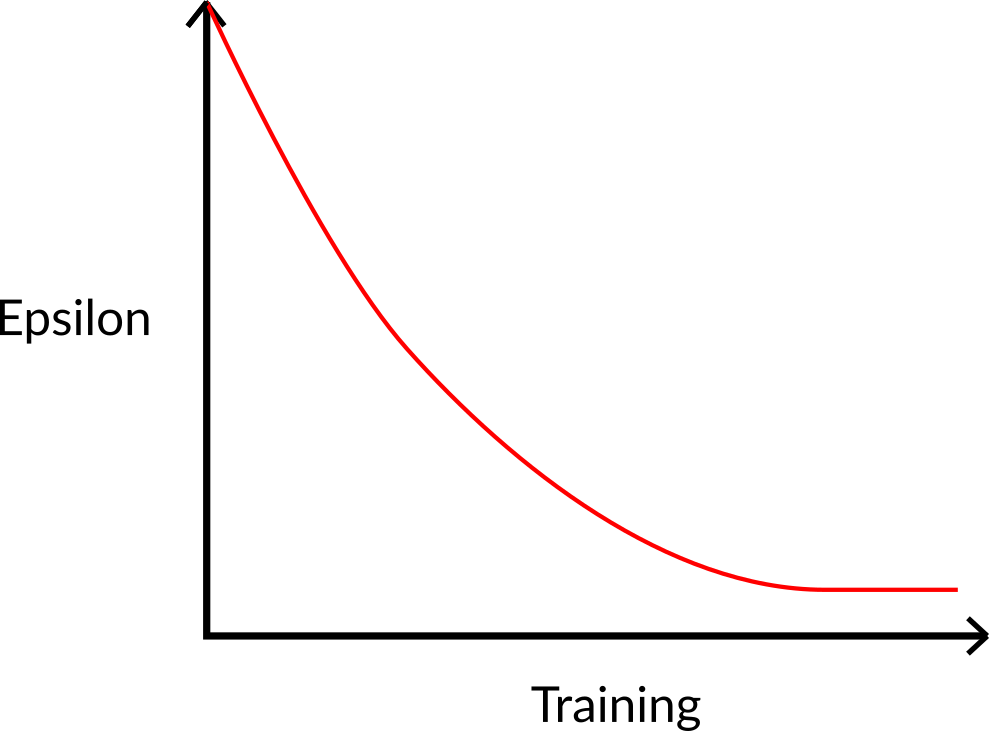
- Step 2: Choose an action using the epsilon-greedy strategy
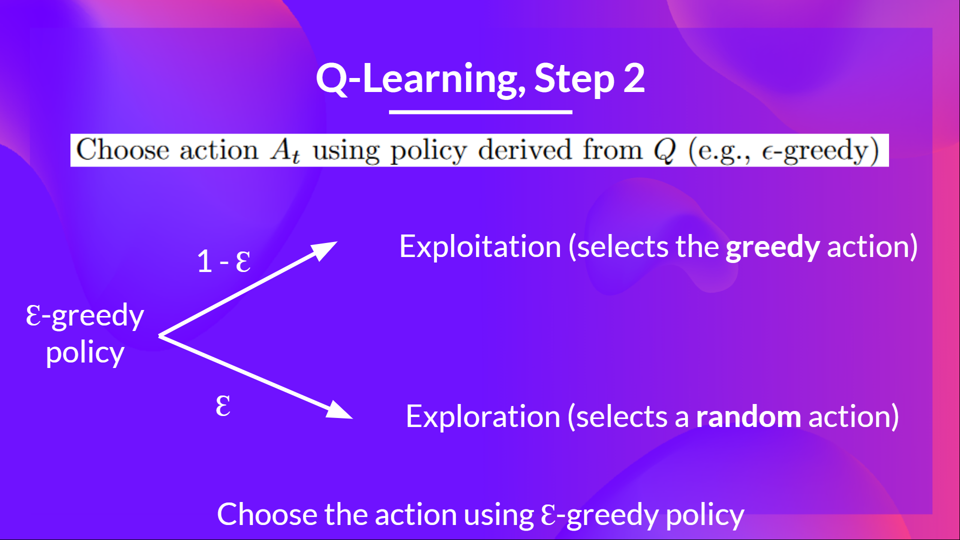
- With probability $\epsilon$, select a random action (exploration).
- With probability $1 - \epsilon$, select the action with the highest Q-value for the current state (exploitation).
- As training progresses, $\epsilon$ is typically decayed to reduce exploration and increase exploitation.
- Step 3: Take the action, observe the reward and the next state, $A_t, R_{t+1}, S_{t+1}$.
- Step 4: Update the Q-value for the current state-action pair using the Q-learning update rule.
- Use the update formula to adjust the Q-value based on the observed reward and the maximum estimated Q-value for the next state.
- To produce the TD target, we use the immediate reward $R_{t+1}$ and the maximum estimated discounted Q-value for the next state $S_{t+1}$ over all possible actions. This is called bootstrapping because we are using our current estimate to improve itself incrementally.
- To get the TD target, we use:
- We obtain the reward $R_{t+1}$ from the environment after taking action $A_t$ in state $S_t$.
- To get the best state-action pair value for the next state $S_{t+1}$, we look at all possible actions $a$ in that state and select the one with the highest Q-value: $\max_a Q(S_{t+1}, a)$ $\rightarrow$ Note that this is not $\epsilon$-greedy; this is always taking the maximum value.
- We multiply this maximum Q-value by the discount factor $\gamma$ to account for the time value of future rewards.
- Finally, we add the immediate reward $R_{t+1}$ to the discounted maximum Q-value to get the TD target: $$\text{TD Target} = R_{t+1} + \gamma \max_a Q(S_{t+1}, a)$$
- Then when the update of this Q-value is done, we start in a new state and select another action using the $\epsilon$-greedy strategy.
- This is why Q-learning is considered an off-policy method because the action used to update the Q-value (the one that maximizes the Q-value for the next state) is not necessarily the action that was actually taken (which could have been a random action due to exploration).
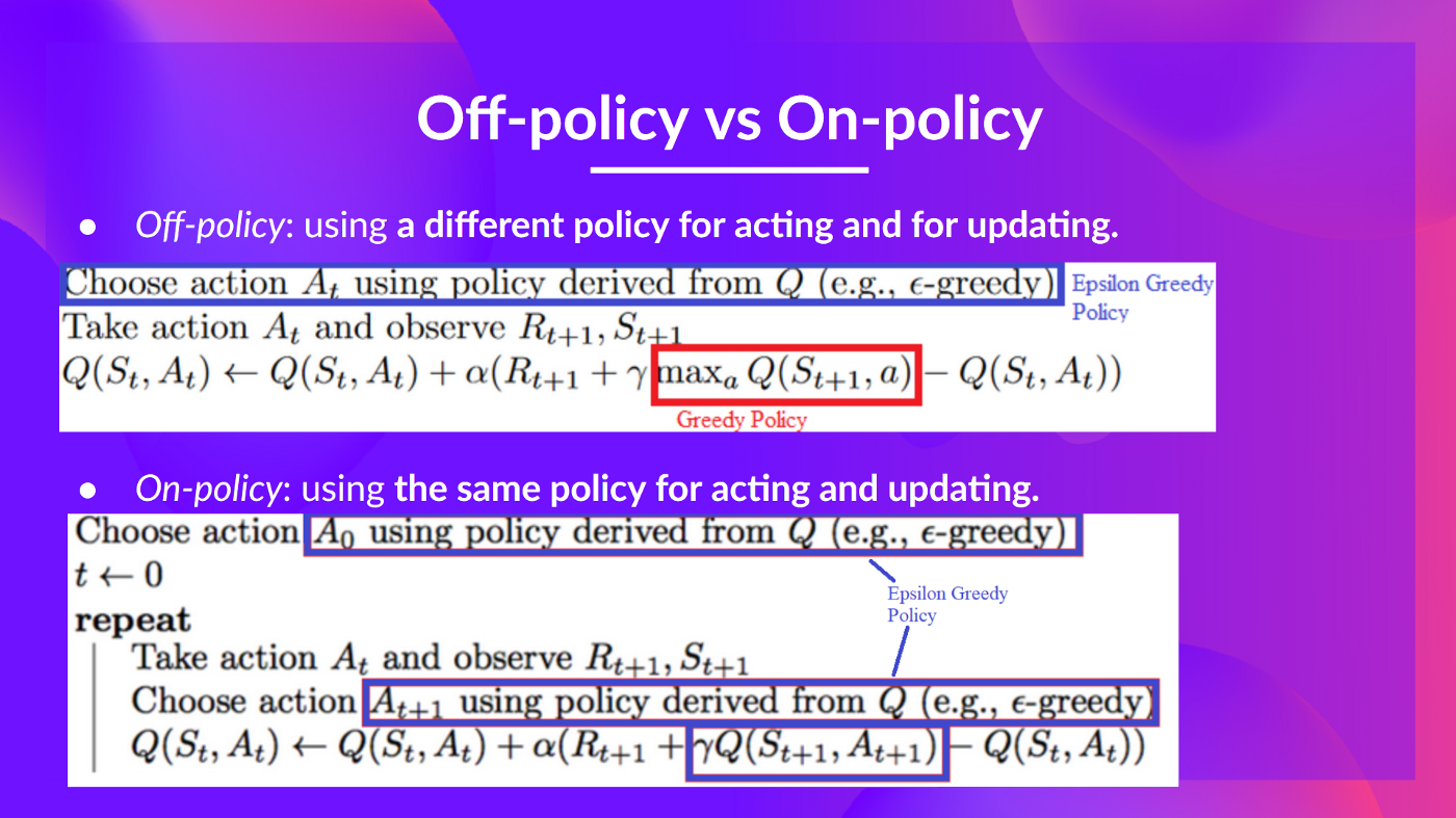
Off-policy vs On-policy
- Off-policy: using a different policy for acting (inference) and learning (training).
- Example: Q-learning $\rightarrow$ uses $\epsilon$-greedy for acting and greedy (max) for learning.
- On-policy: using the same policy for acting and learning.
- Example: SARSA $\rightarrow$ uses $\epsilon$-greedy for both acting and learning.
HFRL Unit-3
- Producing and updating the Q-table becomes challenging in environments with large or continuous state and action spaces.
- Deep Q-Networks (DQN) address this by using neural networks to approximate the Q-function instead of a table.
- DQN uses a neural network to take the state as input and output Q-values for all possible actions.

Q-Function Recap
- The Q-function $Q(s, a)$ is an action-value function that determines the value of being at a particular state and taking a specific action at that state.
- Q-Learning is the algorithm that trains the Q-function.
- “Q” stands for “quality,” representing the quality of a state-action pair in terms of expected cumulative reward.
- Internally Q-function is represented as a Q-table, which maps state-action pairs to their corresponding Q-values.
- Issue: In environments with large or continuous state and action spaces, maintaining and updating a Q-table becomes impractical $\rightarrow$ Qtable doesn’t scale well.
Deep Q-Networks (DQN)
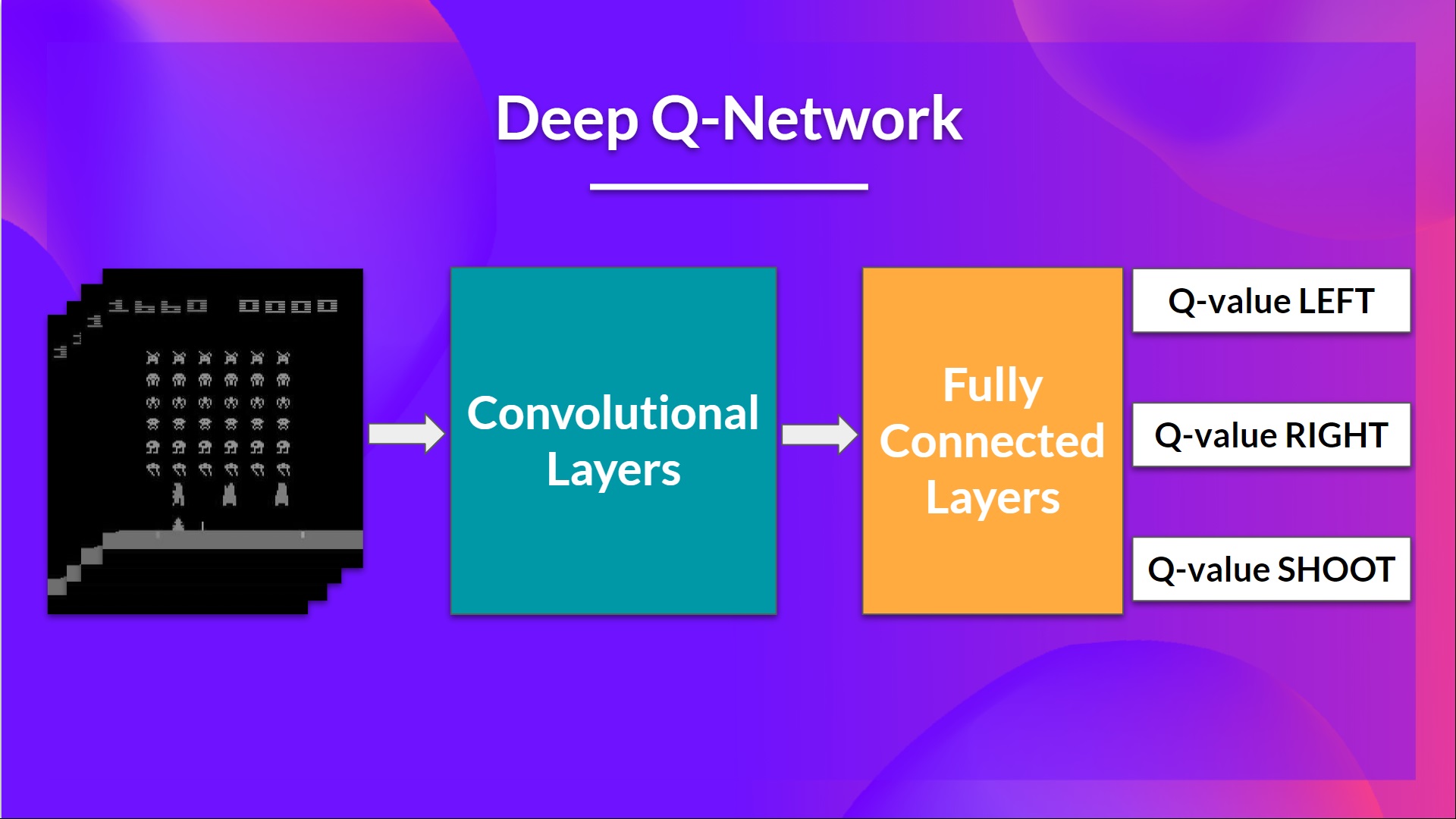
- DQN uses a neural network to approximate the Q-function, allowing it to handle large or continuous state spaces.
- The neural network takes the state as input and outputs Q-values for all possible actions.
- The architecture of a DQN typically includes:
- Input Layer: Receives the state representation (e.g., raw pixels for images).
- Hidden Layers: Multiple fully connected layers with activation functions (e.g., ReLU)
- Output Layer: Outputs Q-values for each possible action.
- The DQN is trained using the Q-learning update rule, but instead of updating a Q-table, we update the weights of the neural network.
- The loss function used for training is based on the difference between the predicted Q-values and the target Q-values (TD target).
- The target Q-values are computed using the immediate reward and the maximum estimated Q-value for the next state, similar to Q-learning
Preprocessing the Input and Temporal Limits

- In environments with high-dimensional inputs (e.g., images), preprocessing is essential to reduce complexity and improve learning efficiency.
- Common preprocessing steps include:
- Grayscaling: Convert RGB images to grayscale to reduce the number of input channels.
- Resizing: Resize images to a smaller, fixed size (e.g., 84x84 pixels), cropping unnecessary parts to focus on relevant information.
- Normalization: Scale pixel values to a range (e.g., [0, 1] or [-1, 1]) to improve training stability.
- Frame Stacking: Stack multiple consecutive frames to provide temporal context, allowing the agent to infer motion and dynamics.
- Temporal limits are imposed on episodes to prevent them from running indefinitely, ensuring that the agent learns to complete tasks within a reasonable time frame.

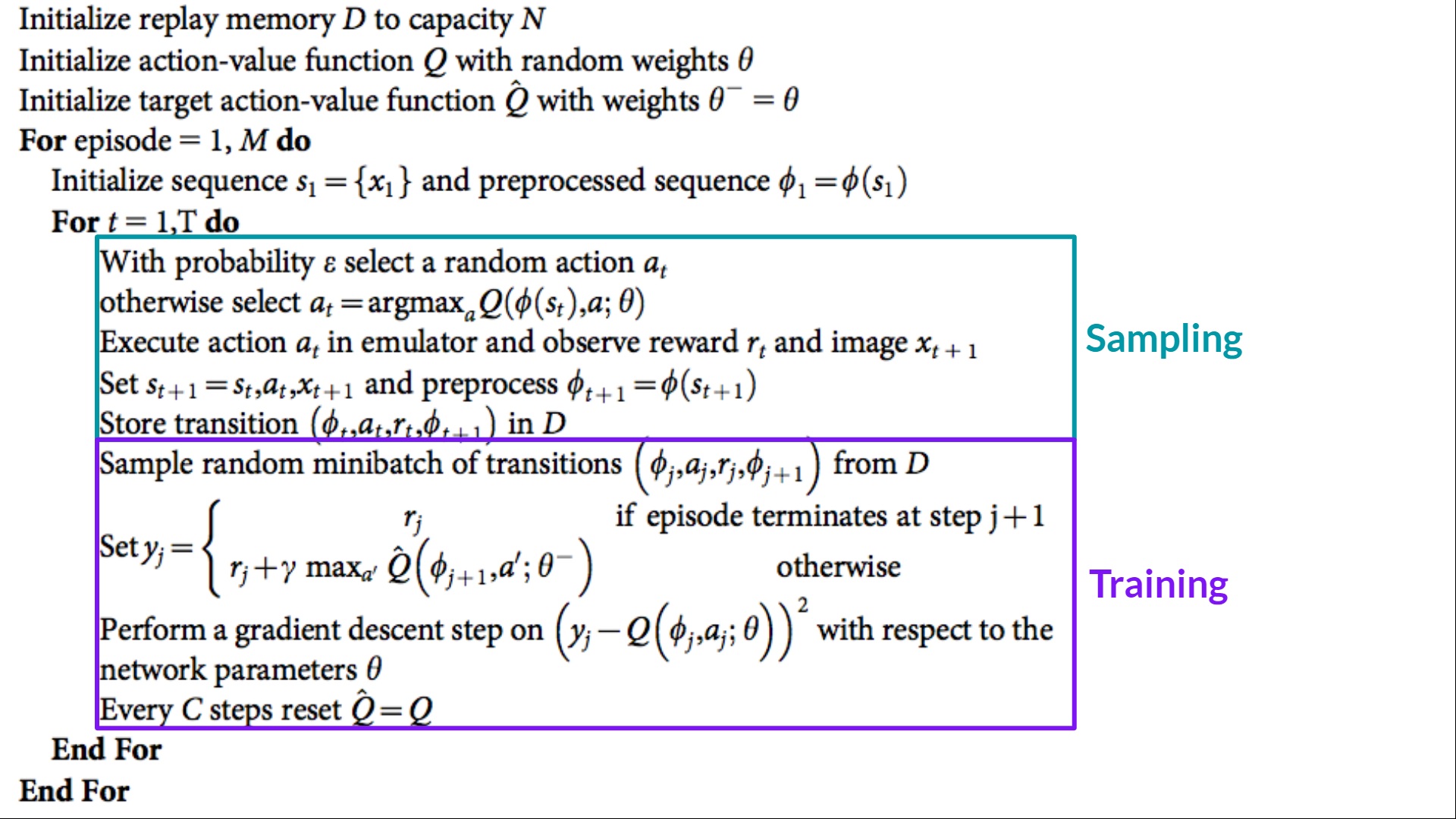
The Deep Q-Learning Algorithm
-
We create a loss function that compares our current Q-value estimates with the Q-target and uses gradient descent to update the Deep Q-Network’s weights to approximate the Q-values better.
-
The Deep Q-Learning algorithm has two phases: the interaction phase and the training phase.
-
Interaction or Sampling Phase:
- The agent performs actions and stores the observed experience tuples in a replay memory.
- Experience tuples typically include the current state, action taken, reward received, and next state.
- This phase allows the agent to explore the environment and gather diverse experiences for training.
-
Training Phase:
- The agent samples mini-batches of experience tuples from the replay memory to train the Deep Q-Network.
- The loss function is computed based on the difference between the predicted Q-values and the target Q-values (TD target).
- The network’s weights are updated using gradient descent to minimize the loss.
- This phase allows the agent to learn from past experiences and improve its policy over time.
- DQN can suffer from instability because of combining a non-linear function approximator (neural network) and bootstrapping (using current estimates to update themselves).
- To address this, DQN uses 3 key techniques:
- Experience Replay to make more efficient use of experiences.
- Fixed Q-Target to stabilize the training.
- Double Deep Q-Learning, to handle the problem of the overestimation of Q-values.
Experience Replay
- Experience Replay stores the agent’s experiences in a replay memory (buffer) and samples mini-batches from this memory to train the network.
- This has two functions:
- Make more efficient use of the experiences during the training. Usually, in online reinforcement learning, the agent interacts with the environment, gets experiences (state, action, reward, and next state), learns from them (updates the neural network), and discards them. This is not efficient. By storing experiences in a replay memory, we can reuse them multiple times for training, improving sample efficiency.
- Avoid forgetting previous experiences (aka catastrophic interference, or catastrophic forgetting) and reduce the correlation between experiences. Catastrophic forgetting happens when the agent learns new information and forgets previously learned information. By sampling randomly from a replay memory, we ensure that the training data is more diverse and less correlated, which helps stabilize learning.
Fixed Q-Target
- We do not know the real TD target because we do not know the optimal Q-values for the next state.
- Bellman equation tells us that the optimal Q-value for the next state is the maximum Q-value over all possible actions in that state.
- Problem: We are using the same parameters (weights) of the neural network to estimate both the current Q-values and the target Q-values. So, there’s significant correlation between the two, which can lead to instability and divergence during training.
- Solution: Use a separate neural network, called the target network, to compute the target Q-values.
- The target network has the same architecture as the main network but with different weights.
- The weights of the target network are updated less frequently (e.g., every few thousand steps) by copying the weights from the main network.
- This decouples the target Q-value estimation from the current Q-value estimation, reducing correlation and improving stability.
- The target Q-value is computed using the target network: $$\text{TD Target} = R_{t+1} + \gamma \max_a Q_{\text{target}}(S_{t+1}, a)$$
- Where $Q_{\text{target}}$ is the Q-value estimated by the target network.
Double Deep Q-Learning
- This handles the problem of the overestimation of Q-values.
- When calculating the target Q-value, we use the main network to select the action that maximizes the Q-value for the next state, but we use the target network to evaluate this action. How are we sure that the best action for the next state is the one that maximizes the Q-value according to the main network? It might be an overestimation.
- The accuracy of the Q-values depends on what action we have tried and what states we have explored.
- If non-optimal actions are regularly given a higher Q value than the optimal best action, the learning will be complicated.
- The solution is to use the Double Q-learning approach:
- Use the DQN network to select the best action that maximizes the Q-value for the next state.
- Use the target network to evaluate this action and compute the target Q-value.
- This reduces the overestimation bias because the action selection and evaluation are decoupled.
- The target Q-value in Double DQN is computed as: $$\text{TD Target} = R_{t+1} + \gamma Q_{\text{target}}(S_{t+1}, \arg\max_a Q_{\text{main}}(S_{t+1}, a))$$
- Where $Q_{\text{main}}$ is the Q-value estimated by the main network, and $Q_{\text{target}}$ is the Q-value estimated by the target network.
Summary of DQN Improvements
| Technique | Purpose | Benefit |
|---|---|---|
| Experience Replay | Store and reuse experiences | Improves sample efficiency and reduces correlation between experiences |
| Fixed Q-Target | Use a separate target network for Q-value estimation | Stabilizes training by reducing correlation between current and target Q-values |
| Double DQN | Decouple action selection and evaluation | Reduces overestimation bias in Q-value estimates |
HFRL Unit-4
Policy-based Methods
-
RL: find optimal policy $\pi^*$ that maximizes expected return.
-
Reward Hypothesis: all goals can be framed as maximizing expected cumulative reward.
-
Two main approaches to find optimal policy:
- Policy-based methods: directly optimize the policy $\pi(a|s)$.
- Value-based methods: learn a value function $V(s)$ or $Q(s, a)$ and derive the policy from it.
- Actor-Critic methods: combine both approaches by learning a policy and a value function simultaneously.
-
In policy based methods we directly learn to approximate the optimal policy $\pi^*$ by adjusting the parameters of the policy to maximize the expected return.
-
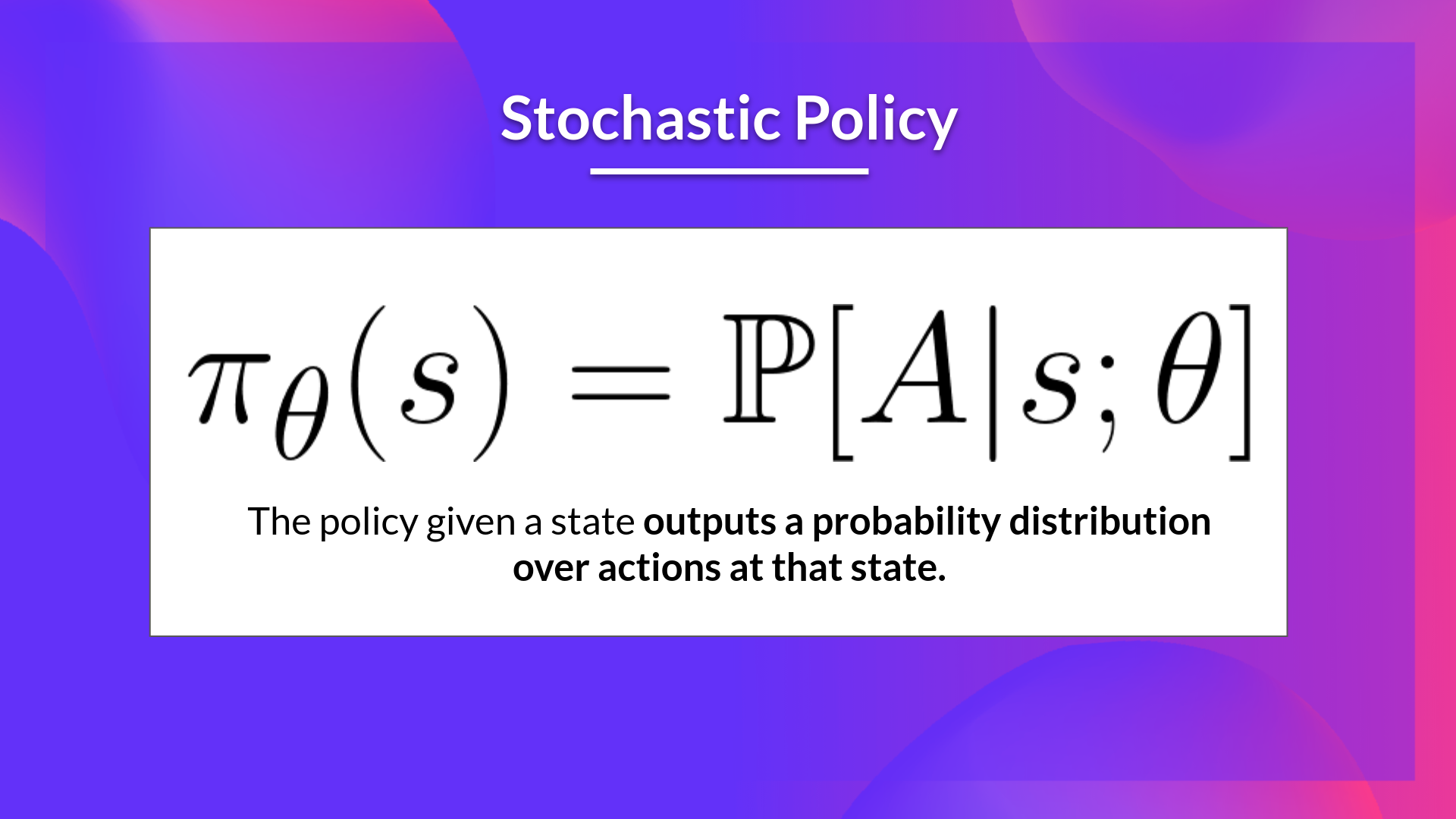
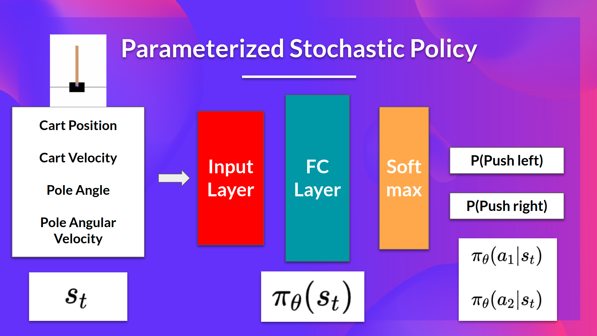
The idea is to parameterize the policy using a neural network, $\pi_\theta$, which will output a probability distribution over actions given a state.
-
We use gradient ascent to update the policy parameters $\theta$ in the direction that increases the expected return.
-
We control the parameter $\theta$ to make the policy better and better over time.
-
We can directly optimize our policy $\pi_\theta$ to output a probability distribution over actions $\pi_\theta(a|s)$ that maximizes the expected return.
-
We define the objective function $J(\theta)$ as the expected return when following the policy $\pi_\theta$:
$$J(\theta) = \mathbb{E}_{\pi_\theta}[G_t]$$ -
Where $G_t$ is the return (cumulative discounted reward) from time step $t$.
-
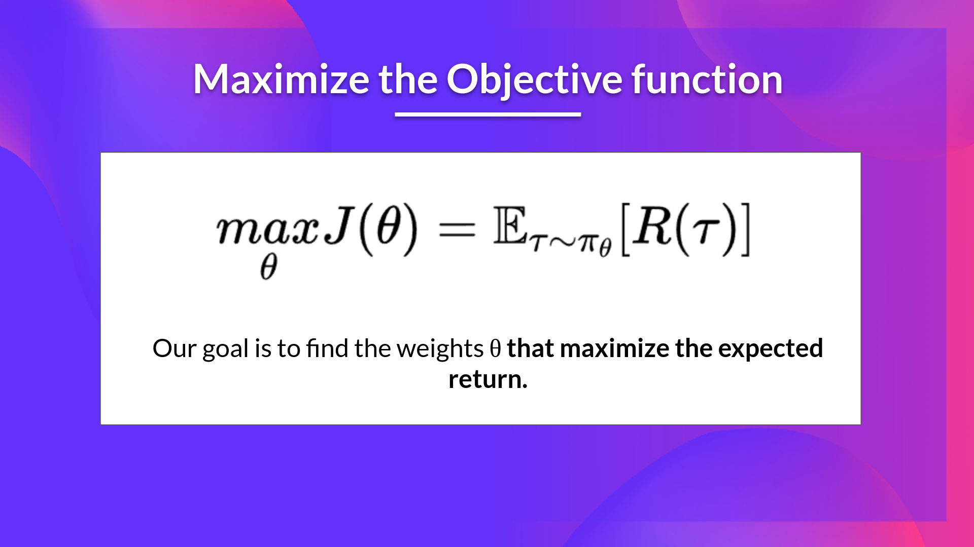
The goal is to find the optimal parameters $\theta^*$ that maximize $J(\theta)$:
$$\theta^* = \arg\max_\theta J(\theta)$$ -
We use gradient ascent to update the policy parameters $\theta$:
$$\theta \leftarrow \theta + \alpha \nabla_\theta J(\theta)$$ -
Where $\alpha$ is the learning rate, and $\nabla_\theta J(\theta)$ is the gradient of the objective function with respect to the policy parameters $\theta$.
-
The difference between Policy-based and policy-gradient methods
- Policy-based methods refer to a broader category of RL algorithms that directly optimize the policy $\pi(a|s)$ to maximize the expected return.
- Policy-gradient methods are a specific type of policy-based methods that use gradient ascent to update the policy parameters $\theta$ based on the gradient of the objective function $J(\theta)$.
- In summary, all policy-gradient methods are policy-based methods, but not all policy-based methods are policy-gradient methods.
Why use policy-based methods?
- The simplicity of integration $\rightarrow$ directly optimize the policy without needing to learn a value function.
- Learn stochastic policies $\rightarrow$ can learn policies that output a probability distribution over actions, allowing for exploration and handling uncertainty.
- No perceptual aliasing $\rightarrow$ Perceptual aliasing is when two states seem (or are) the same but need different actions.
- Value-based methods can struggle with this because they rely on the value function, which may not distinguish between these states as they are quasi-greedy in nature.
- Policy-based methods can learn different actions for these states directly through the policy.
- More efficient in high-dimensional or continuous action spaces $\rightarrow$ Value-based methods can struggle with large or continuous action spaces because they need to estimate the value for each state-action pair.
- Policy-based methods can directly output actions without needing to evaluate all possible actions.
- Better convergence properties $\rightarrow$ Policy-based methods can have better convergence properties in some scenarios, especially when the policy is stochastic.
- Stochastic policy action preferences change smoothly, leading to more stable learning.
Disadvantages of Policy-based methods
- Convergence to local optima $\rightarrow$ Policy-gradient methods can converge to local optima, especially in complex environments with many suboptimal policies.
- High variance in gradient estimates $\rightarrow$ The gradient estimates used in policy-gradient methods can have high variance, leading to unstable learning.
- Slower learning $\rightarrow$ Policy-based methods can be slower to learn compared to value-based methods, especially in environments with sparse rewards.
Policy Gradient Methods
- Find parameters $\theta$ of a policy $\pi_\theta(a|s)$ that maximizes the expected return $J(\theta)$.
- Outputs a probability distribution over actions given a state.
- The probability of taking action $a$ in state $s$ is given by $\pi_\theta(a|s)$ $\rightarrow$ known as action preference.
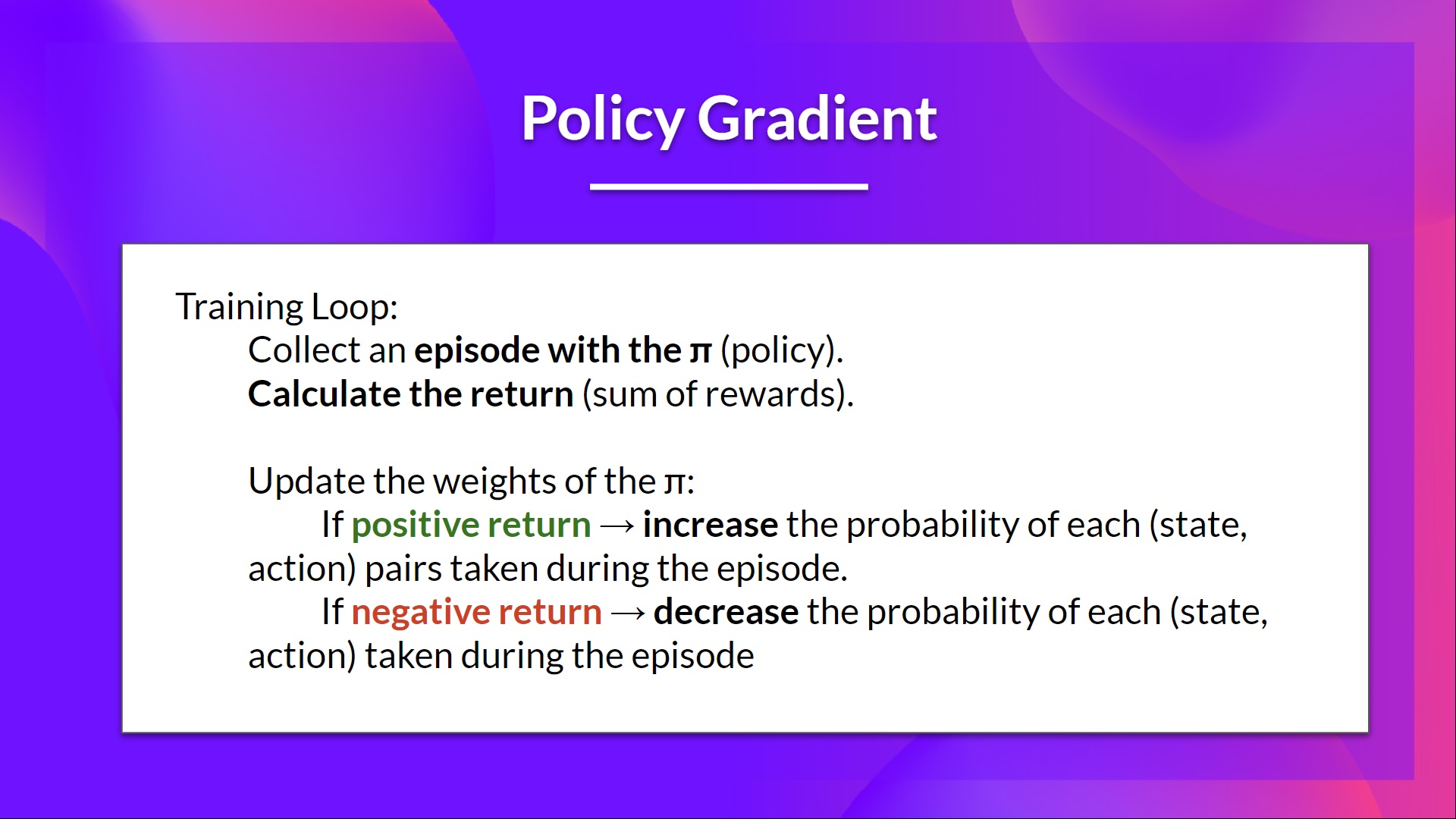
Goal: Control the probability distribution of actions by tuning the policy so that good actions are more likely to be chosen.
- Let the agent interact with the environment using its current policy $\pi_\theta$ and collect experiences (state, action, reward, next state).
- If the action taken leads to a high reward, we want to increase the probability of taking that action in that state.
- For each state-action pair $(s,a)$, we want to increase the probability $\pi_\theta(a|s)$ if the action $a$ taken in state $s$ leads to a high return.
- Conversely, if the action taken leads to a low reward, we want to decrease the probability of taking that action in that state.
- Stochastic policy $\pi_\theta(a|s)$: outputs a probability distribution over actions given a state.
- How to know if our policy is good $\rightarrow$ we need a way to evaluate the quality of our policy.
- We define the objective function $J(\theta)$ as the expected return when following the policy $\pi_\theta$.
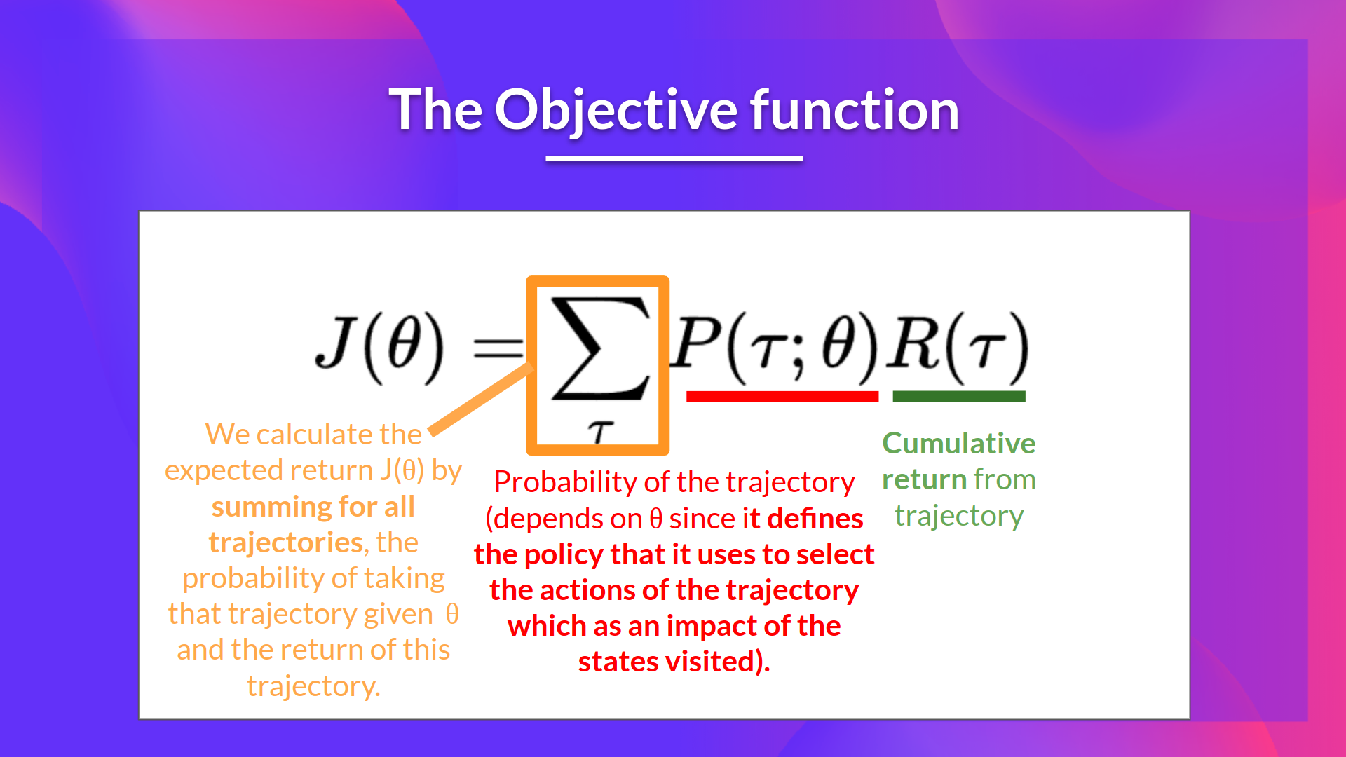
- Measures the performance of the agent given a trajectory $\tau$ (sequence of states, actions) and outputs a scalar value representing the expected return.
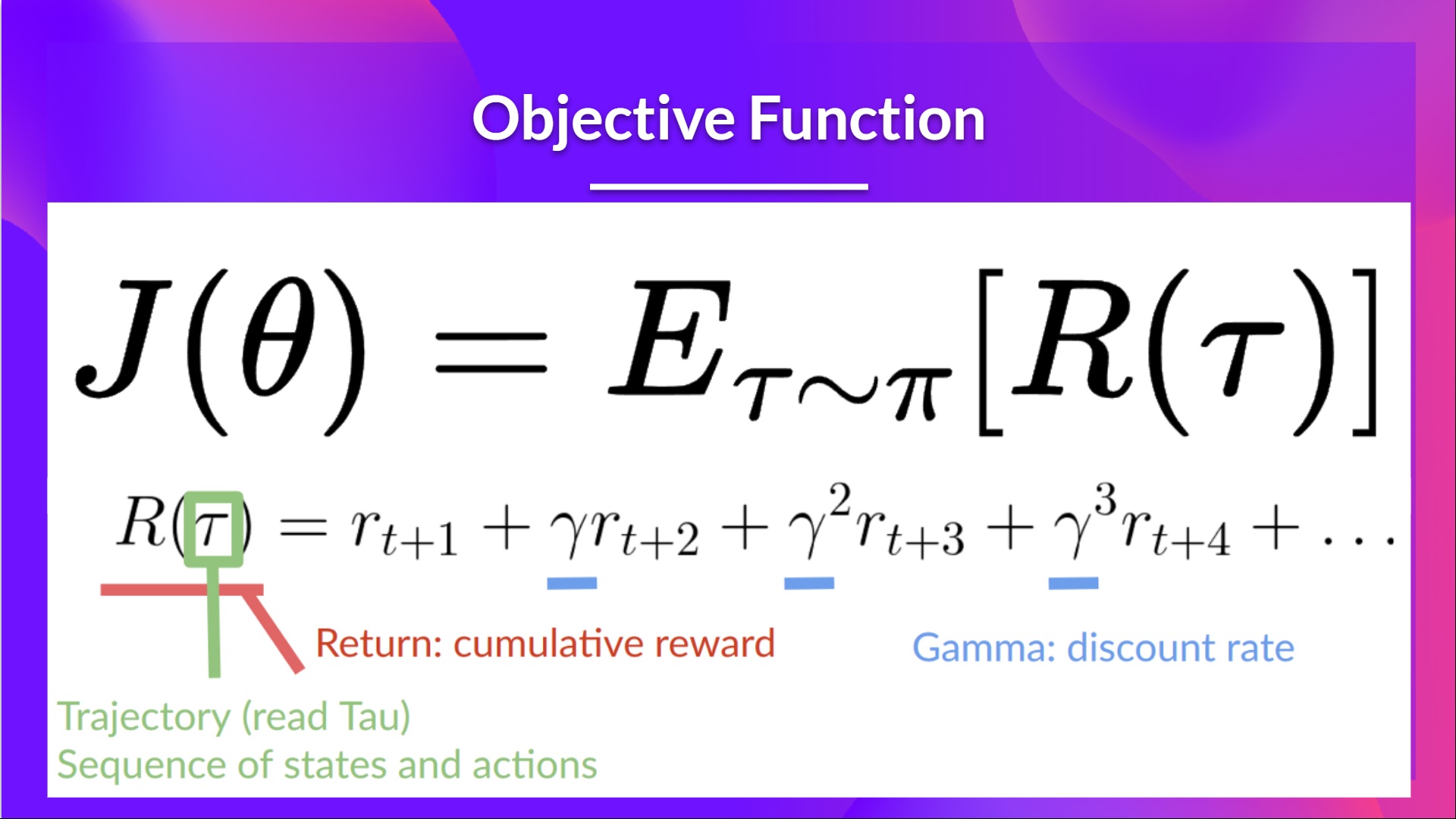
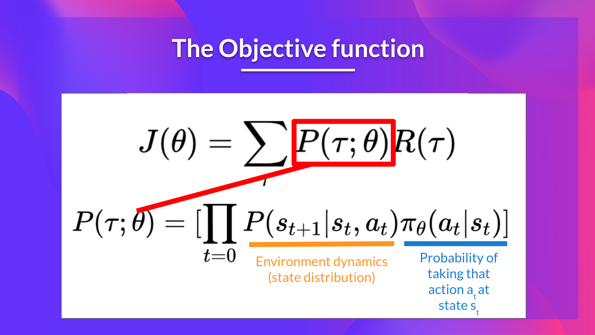
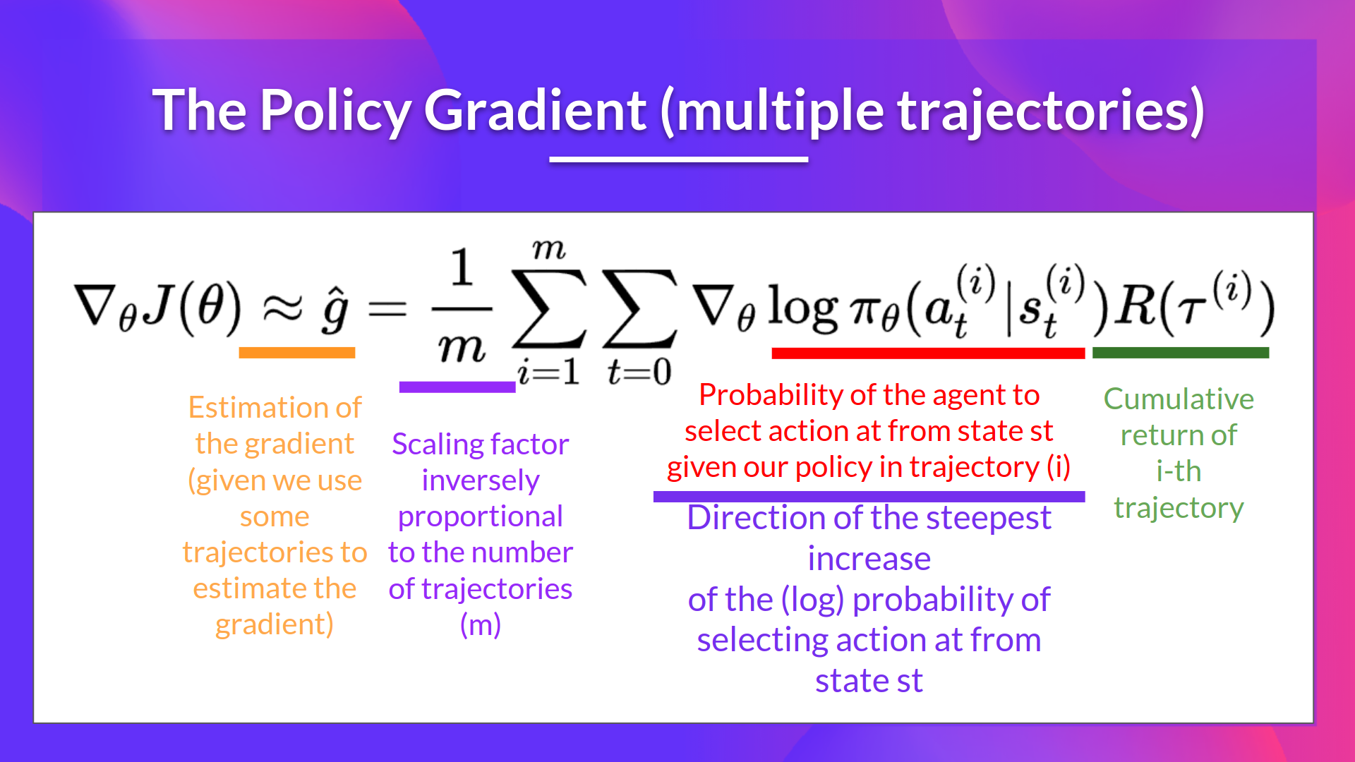
- The expected return (also called expected cumulative reward), is the weighted average (where the weights are given by $P(\tau; \theta)$) of the returns $R(\tau)$ over all possible trajectories $\tau$ that can be generated by following the policy $\pi_\theta$.
- $R(\tau)$ is the return (cumulative discounted reward) obtained by following an arbitrary trajectory $\tau$. We need to multiply it by the probability of that trajectory occurring under the current policy, $P(\tau; \theta)$ to get the expected return.
- $P(\tau; \theta)$ is the probability of observing a trajectory $\tau$ when following the policy $\pi_\theta$. This probability depends on the policy parameters $\theta$ because the policy determines the actions taken at each state, which in turn affects the trajectory.
- $J(\theta)$ is the expected return when following the policy $\pi_\theta$. We calculate it by summing over all possible trajectories $\tau$, multiplying the return $R(\tau)$ for each trajectory by its probability $P(\tau; \theta)$.
- The goal of policy-gradient methods is to find the optimal parameters $\theta^*$ that maximize the objective function $J(\theta)$: $$\theta^* = \arg\max_\theta J(\theta)$$
Gradient Ascent and the Policy Gradient Theorem
- We want to find the optimal parameters $\theta^*$ that maximize the objective function $J(\theta)$.
- It’s inverse of gradient descent (used in supervised learning) because we want to maximize the objective function instead of minimizing it.
- Update step for gradient ascent: $$\theta \leftarrow \theta + \alpha \times \nabla_\theta J(\theta)$$
- Where $\alpha$ is the learning rate, and $\nabla_\theta J(\theta)$ is the gradient of the objective function with respect to the policy parameters.
- The gradient $\nabla_\theta J(\theta)$ tells us how to change the policy parameters $\theta$ to increase the expected return $J(\theta)$.
- Two problems with computing the gradient $\nabla_\theta J(\theta)$:
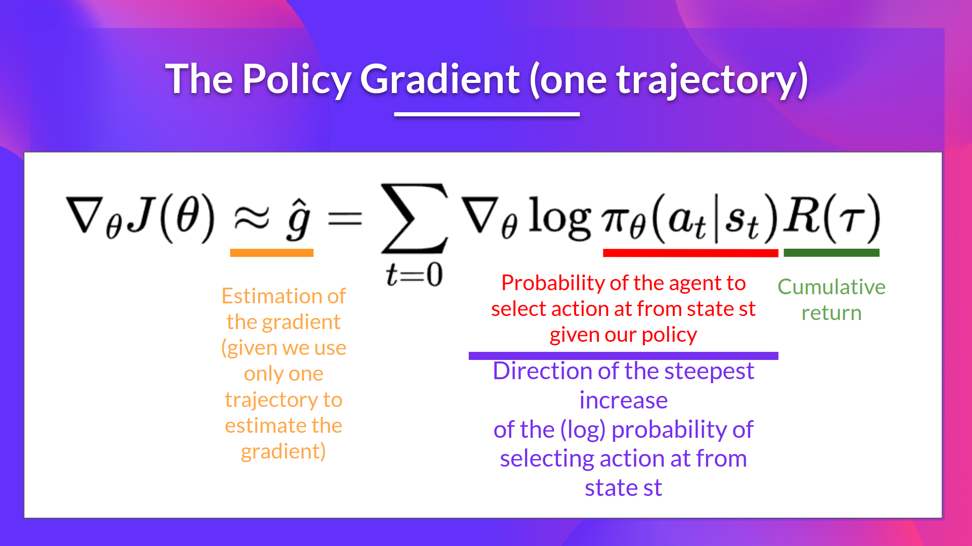
- We cannot calculate the true gradient of the objective function as it requires calculating the probability of each possible trajectory, which is infeasible in complex environments. So we calculate a gradient estimation with a sample-based estimate by collecting a batch of trajectories by interacting with the environment using the current policy $\pi_\theta$.
- To differentiate this objective function we have to differentiate the state distribution which is a Markov Decision Process (MDP) and it’s dependent of the environment dynamics which we don’t know.
- To solve these, we use the Policy Gradient Theorem to derive a more practical expression for the gradient that does not depend on the state distribution.
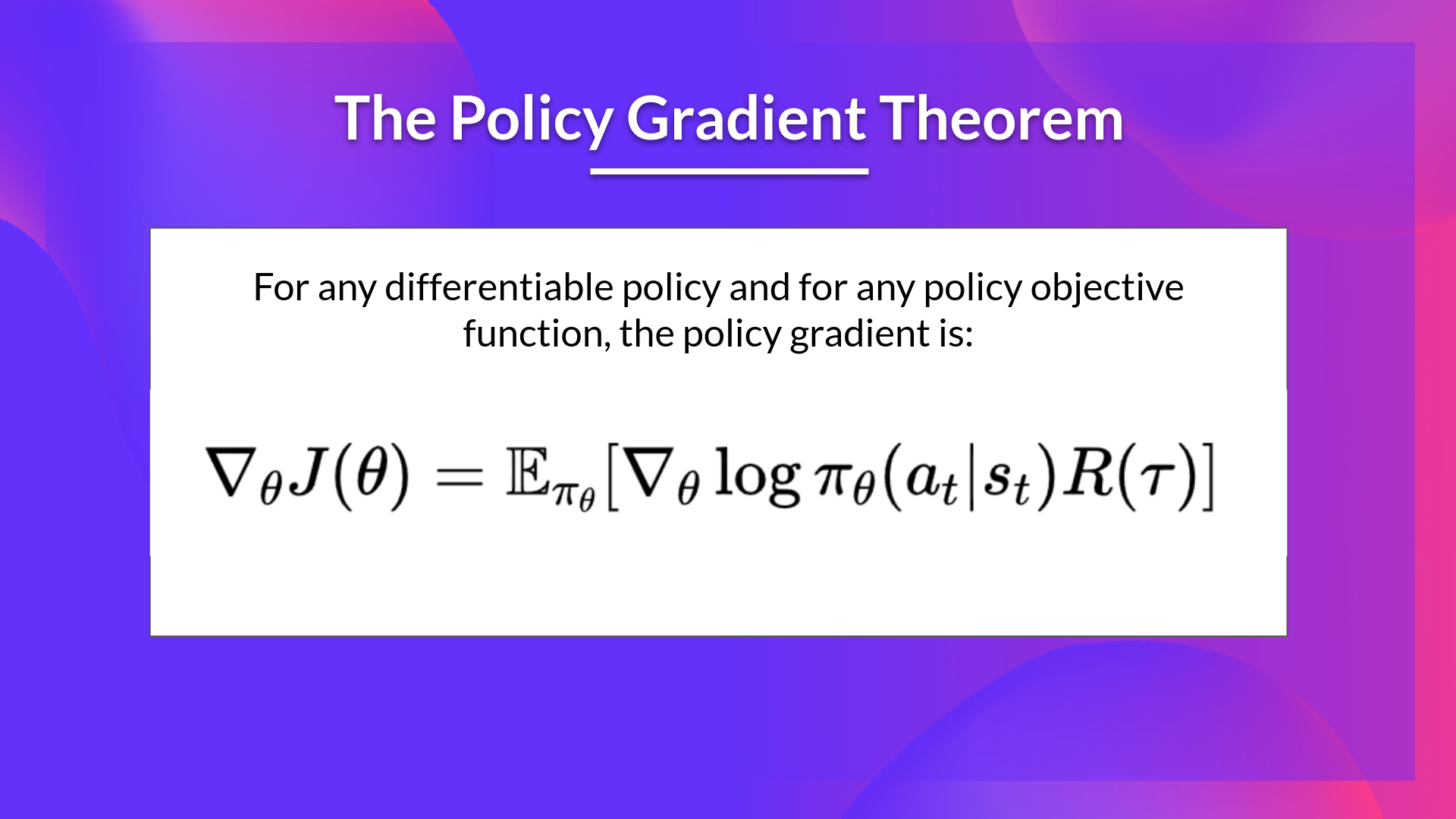
The REINFORCE Algorithm
- REINFORCE is a Monte Carlo policy-gradient algorithm that uses the policy gradient theorem to estimate the gradient of the objective function.
- It collects complete episodes (trajectories) by interacting with the environment using the current policy $\pi_\theta$.
- For each time step $t$ in the episode, it computes the return $G_t$ (cumulative discounted reward) from time step $t$ to the end of the episode.
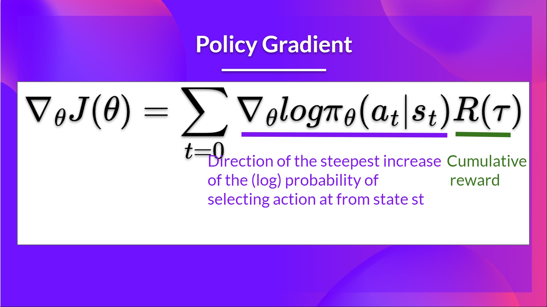
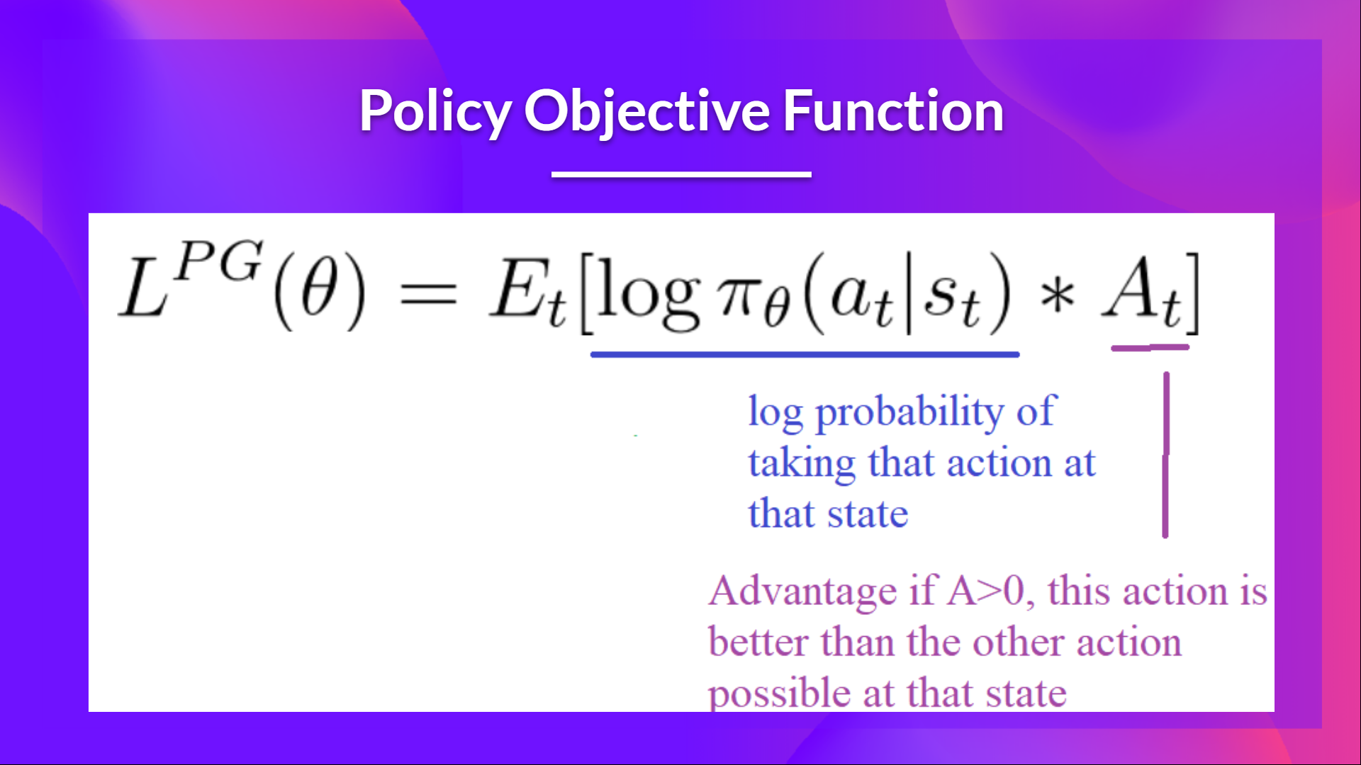
- The policy parameters $\theta$ are updated using the following update rule: $$\theta \leftarrow \theta + \alpha \times G_t \times \nabla_\theta \log \pi_\theta(A_t | S_t)$$
- Where $\alpha$ is the learning rate, $G_t$ is the return from time step $t$, and $\nabla_\theta \log \pi_\theta(A_t | S_t)$ is the gradient of the log-probability of the action taken at time step $t$.
- The term $G_t \times \nabla_\theta \log \pi_\theta(A_t | S_t)$ is known as the policy gradient estimate.
- The REINFORCE algorithm can be summarized in the following steps:
- Initialize the policy parameters $\theta$ randomly.
- For each episode:
- Collect a trajectory by interacting with the environment using the current policy $\pi_\theta$.
- For each time step $t$ in the episode:
- Compute the return $G_t$ from time step $t$ to the end of the episode.
- Update the policy parameters $\theta$ using the update rule.
- Repeat until convergence.
HFRL Unit-5
SKIP – FOR NOW – NOT NEEDED
HFRL Unit-6
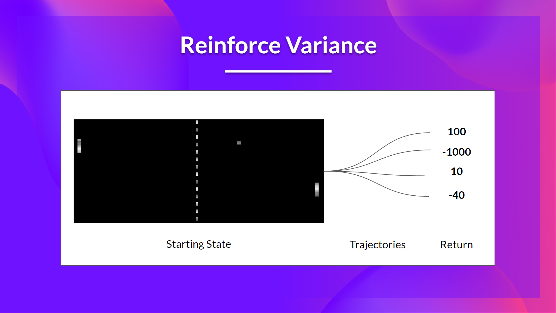
- REINFORCE has high variance in its gradient estimates, leading to unstable learning.
- This high variance arises because we are using Monte Carlo estimates of the return $G_t$, which can vary significantly between episodes.
- Policy gradient estimation is the direction of the steepest ascent in the policy parameter space that maximizes the expected return.
- In Monte Carlo methods like REINFORCE, we estimate the policy gradient using complete episodes, which can lead to high variance in the estimates. We need a lot of samples (episodes) to get a reliable estimate of the gradient.
- Actor-Critic methods combine policy-based and value-based approaches to reduce the variance in policy gradient estimates.
- In this approach, we have two components:
- Actor: The policy network $\pi_\theta(a|s)$ that outputs a probability distribution over actions given a state.
- Critic: The value network $V_w(s)$ that estimates the value of a state.
- Advantage Actor-Critic is an extension of the Actor-Critic method that uses the advantage function to reduce variance further.
The Problem of High Variance in REINFORCE
-
In REINFORCE, we want to increase the probability of actions that lead to high returns and decrease the probability of actions that lead to low returns.
-
The return $R(\tau)$ is calculated using Monte Carlo sampling.
-
We collect a trajectory $\tau$ by interacting with the environment using the current policy $\pi_\theta$.
-
The return $R(\tau)$ is the cumulative discounted reward obtained by following the trajectory $\tau$.
-
If the return is good, all actions will be “reinforced” by increasing their likelihood of being chosen in the future.
-
This method is unbiased as we are using the true return $R(\tau)$ to update the policy.
-
However, because of stochasticity in the environment and the policy, the return $R(\tau)$ can vary significantly between episodes, leading to high variance in the policy gradient estimates.
-
High variance in the gradient estimates can lead to unstable learning and slow convergence.
Advantage Actor-Critic (A2C)
- Actor-Critic methods address the high variance problem by introducing a value function (the Critic) to estimate the expected return.
- We have two function approximators:
- Actor: The policy network $\pi_\theta(a|s)$ that outputs a probability distribution over actions given a state.
- Critic: The value network $V_w(s)$ that estimates how good the action taken in a state is.
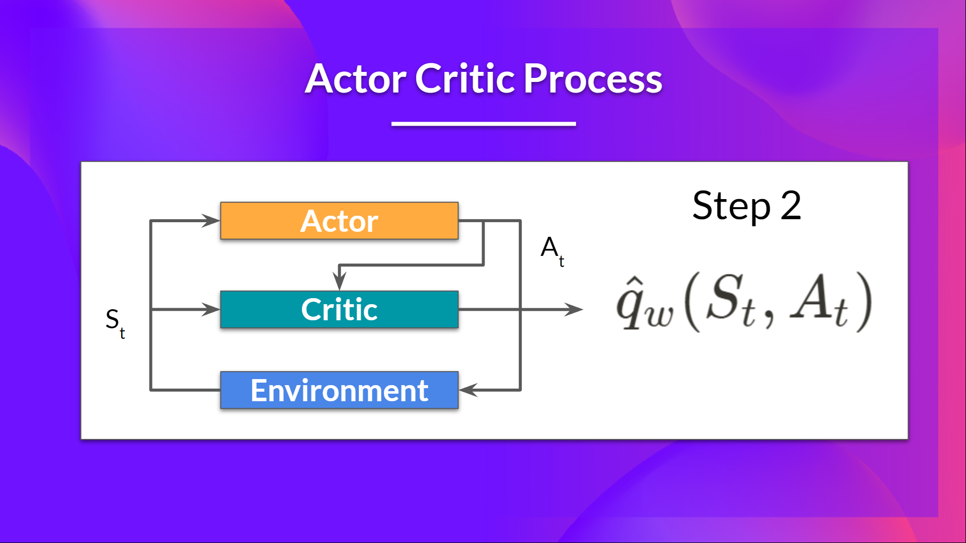
Actor Critic Process
- Actor: a policy function parameterized by $\theta$: $\pi_\theta(s)$
- Critic: a value function parameterized by $w$: $\hat{q}_w(s, a)$
- At each timestep $t$, we get the current state $S_t$ from the environment and pass it to the Actor and Critic networks.
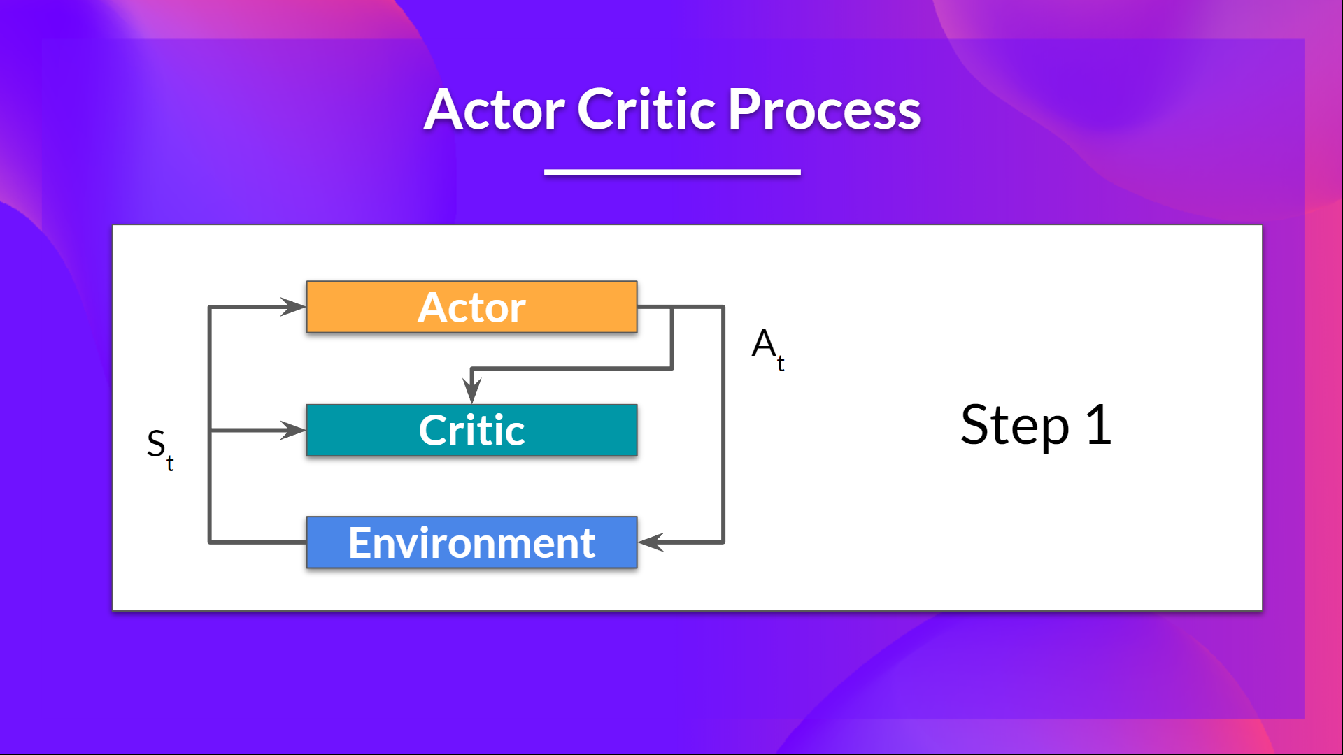
- Our policy takes the state and outputs an action $A_t$.
- The critic takes that action also as an input and using the state $S_t$ along with the action $A_t$ outputs an estimate of the value of taking that action in that state: $\hat{q}_w(S_t, A_t) \rightarrow Q$ estimate.
- We take that action $A_t$ and pass it to the environment, which returns the next state $S_{t+1}$ and the reward $R_{t+1}$.
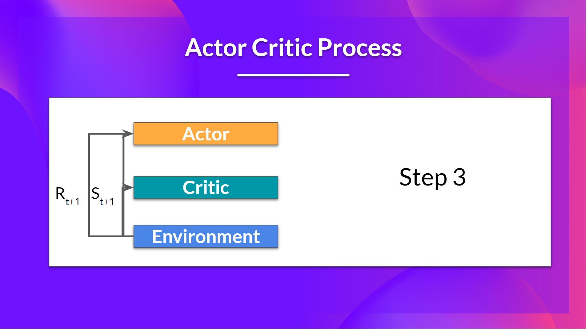
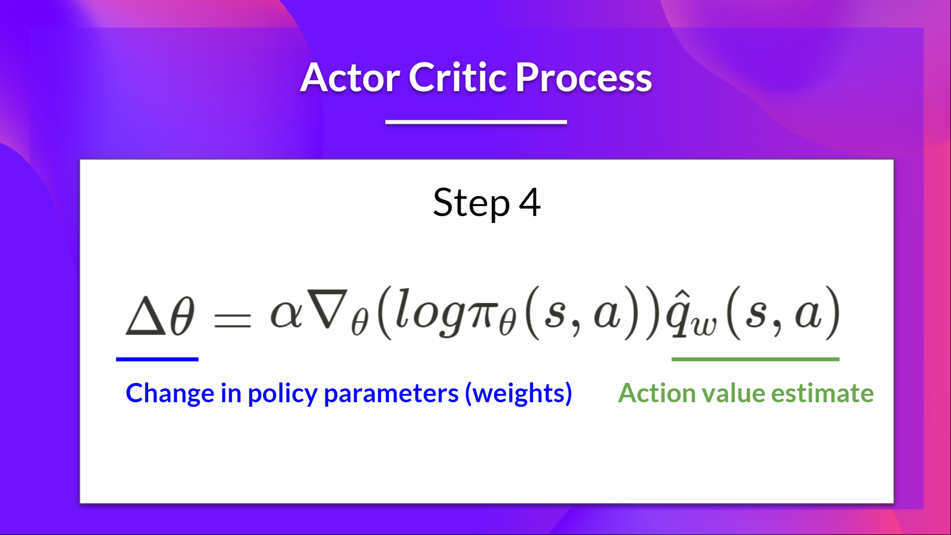
- The Actor updates its policy parameters $\theta$ using the Q-value estimate from the Critic.
- The Actor produces the next action $A_{t+1}$ based on the next state $S_{t+1}$.
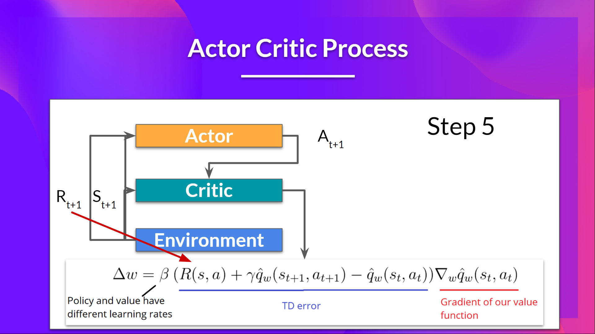
- The Critic updates its value function parameters $w$ using the TD error.
Adding Advantage in Actor-Critic
- Instead of using the Q-value estimate $\hat{q}_w(S_t, A_t)$ directly, we can use the advantage function to reduce variance further.
- The advantage function $A(s, a)$ measures how much better taking action $a$ in state $s$ is compared to the average action in that state.
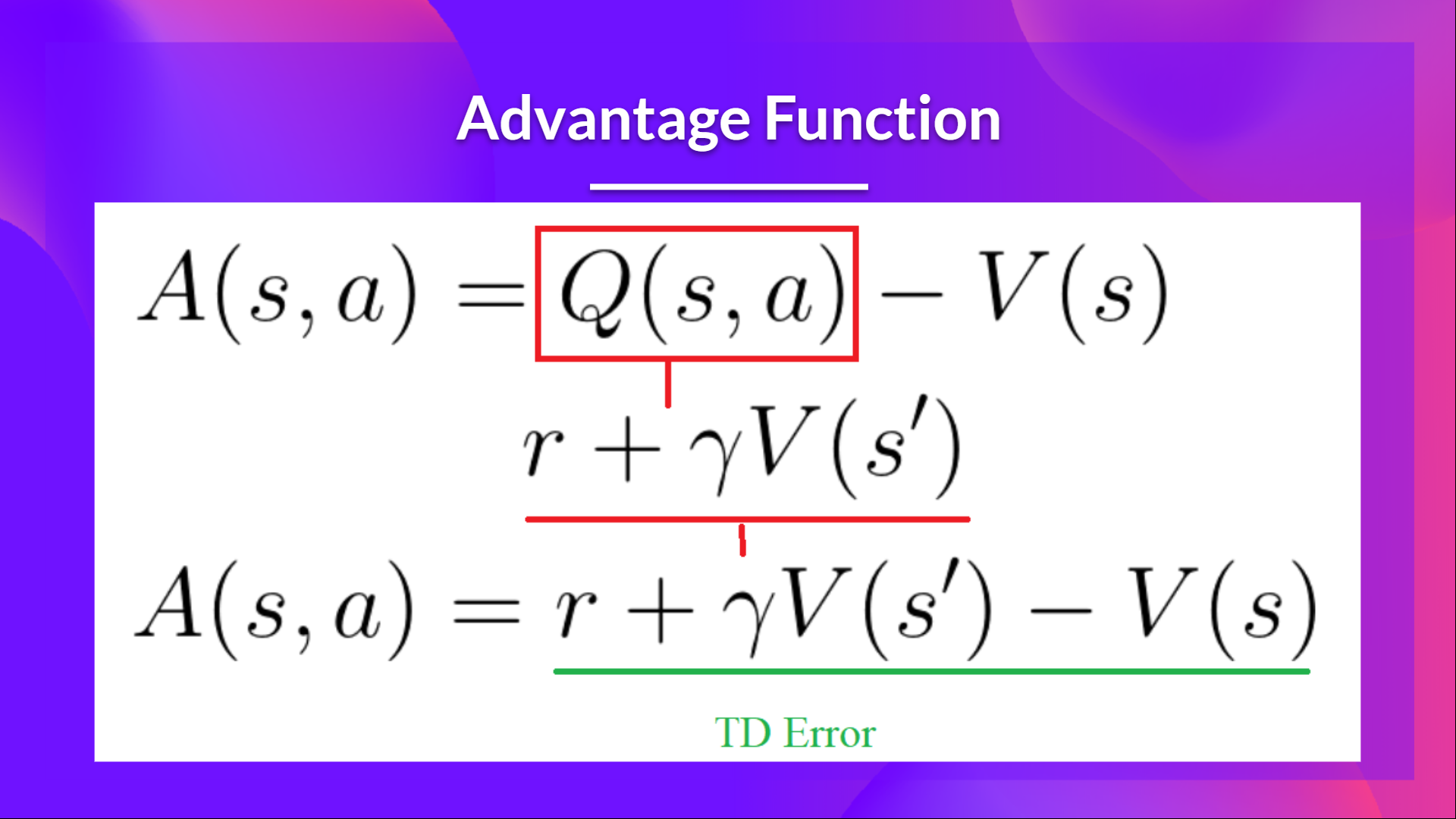
- The advantage function is defined as: $$A(s, a) = Q(s, a) - V(s)$$
- Where $Q(s, a)$ is the action-value function, and $V(s)$ is the state-value function.
- In Advantage Actor-Critic, we use the advantage function to update the policy parameters $\theta$: $$\theta \leftarrow \theta + \alpha \times A(S_t, A_t) \times \nabla_\theta \log \pi_\theta(A_t | S_t)$$
- Where $A(S_t, A_t)$ is the advantage estimate for the action taken at time step $t$.
- The advantage estimate can be computed using the TD error: $$A(S_t, A_t) = R_{t+1} + \gamma V_w(S_{t+1}) - V_w(S_t)$$
- Where $R_{t+1}$ is the immediate reward, $\gamma$ is the discount factor, and $V_w(S_{t+1})$ and $V_w(S_t)$ are the value estimates from the Critic network.
HFRL Unit-7
- SKIP – FOR NOW – NOT NEEDED
HFRL Unit-8
- Proximal Policy Optimization is an architecture that improves the RL agent’s training stability by avoiding policy updates that are too large.
- To do that we use a ratio that indicates the difference between our current policy and old policy and clip this ratio to a range of $[1 - \epsilon, 1 + \epsilon]$.
The Intuition Behind PPO
-
We want to stablize the training of the policy by avoiding large updates that can lead to instability.
-
Reasons:
- Smaller updates lead to more stable learning and more likely convergence to a good policy.
- Large updates can lead to divergence, falling off the cliff, and unstable learning, leading to poor performance and too long to converge.
-
To update policy conservatively, we measure how much the current policy changed compared to the former one using a ratio calculation between the current policy and the old policy.
-
We clip this ratio to a range of $[1 - \epsilon, 1 + \epsilon]$ to limit the change in the policy.
-
This is why it’s called Proximal Policy Optimization $\rightarrow$ we are optimizing the policy while keeping it close to the old policy (proximal).
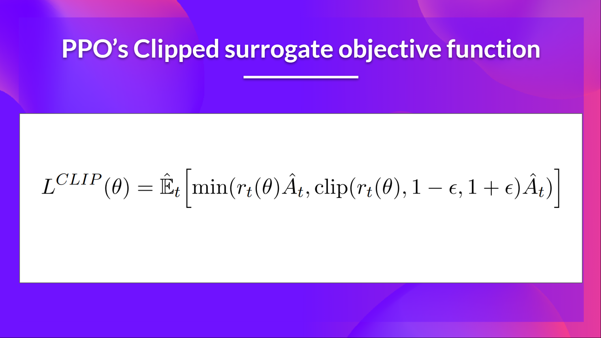
The PPO Objective Function – Clipped Surrogate Objective
- The objective function for PPO is called the clipped surrogate objective.
- This constrain the policy change in small range using a clipping mechanism.
The Ratio Function
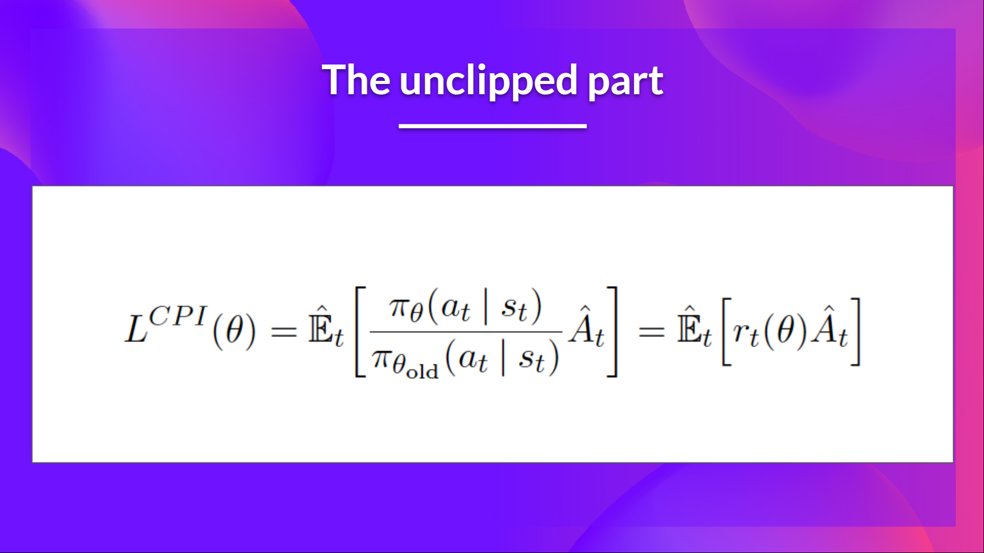
- $r_t(\theta) = \frac{\pi_\theta(a_t | s_t)}{\pi_{\theta_{old}}(a_t | s_t)}$
- The ratio function $r_t(\theta)$ measures how much the current policy $\pi_\theta(a_t | s_t)$ differs from the old policy $\pi_{\theta_{old}}(a_t | s_t)$ for the action $a_t$ taken in state $s_t$
- If the ratio is close to 1, it means the current policy is similar to the old policy for that action.
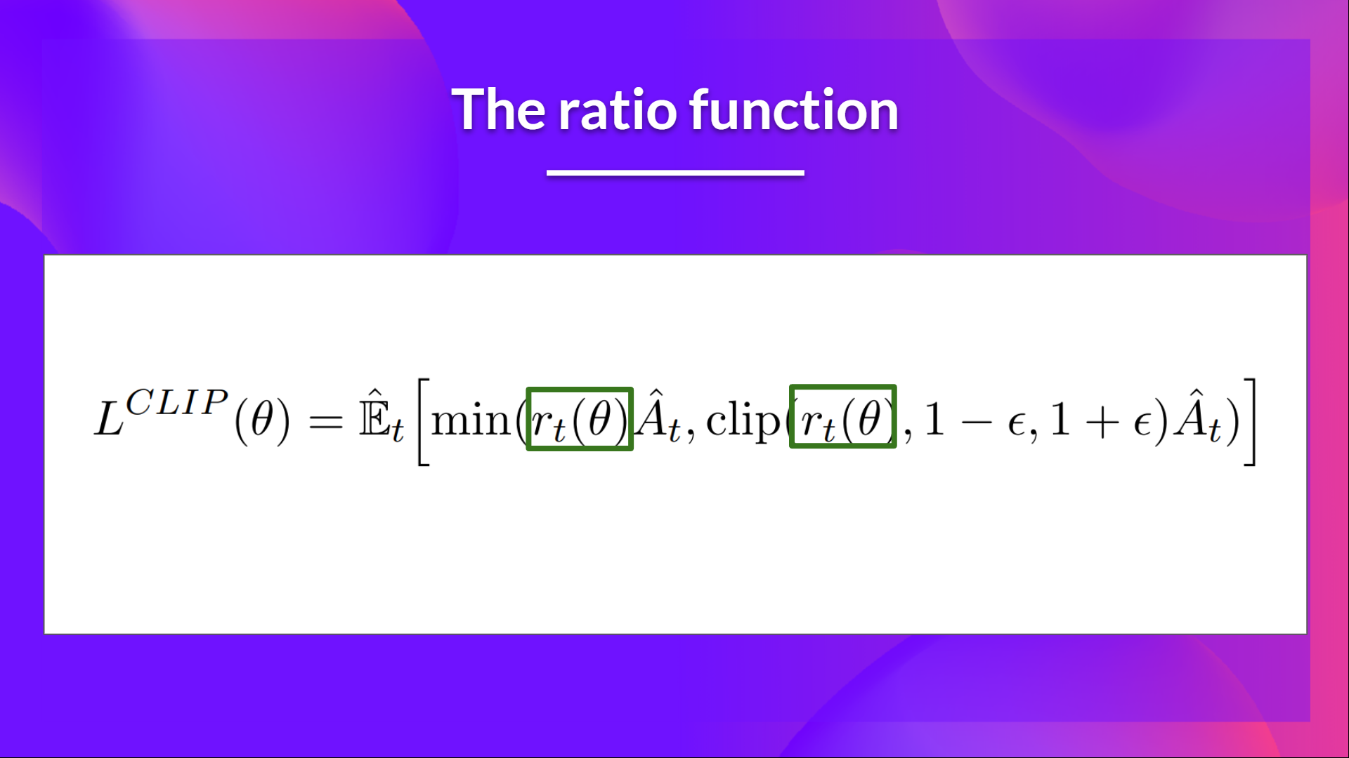
- If the ratio is greater than 1, it means the current policy is more likely to take that action compared to the old policy.
- If the ratio is less than 1, it means the current policy is less likely to take that action compared to the old policy.
- The ratio function is used to measure the change in the policy for the action taken at time step $t$.

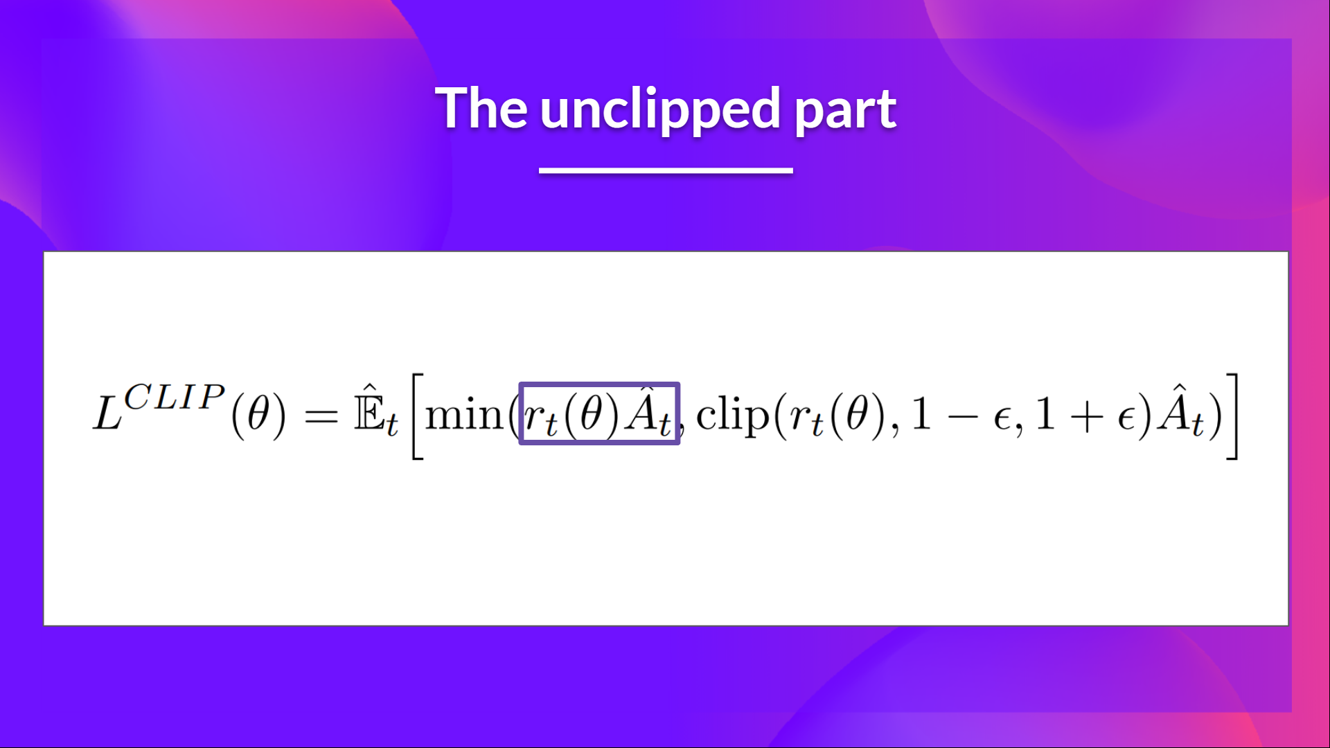
The Unclipped Objective
- The ratio function, $r_t(\theta)$, is multiplied by the advantage estimate, $A_t$, to form the unclipped objective.
- Here the ratio function takes the place of the log-probability used in REINFORCE and Advantage Actor-Critic.
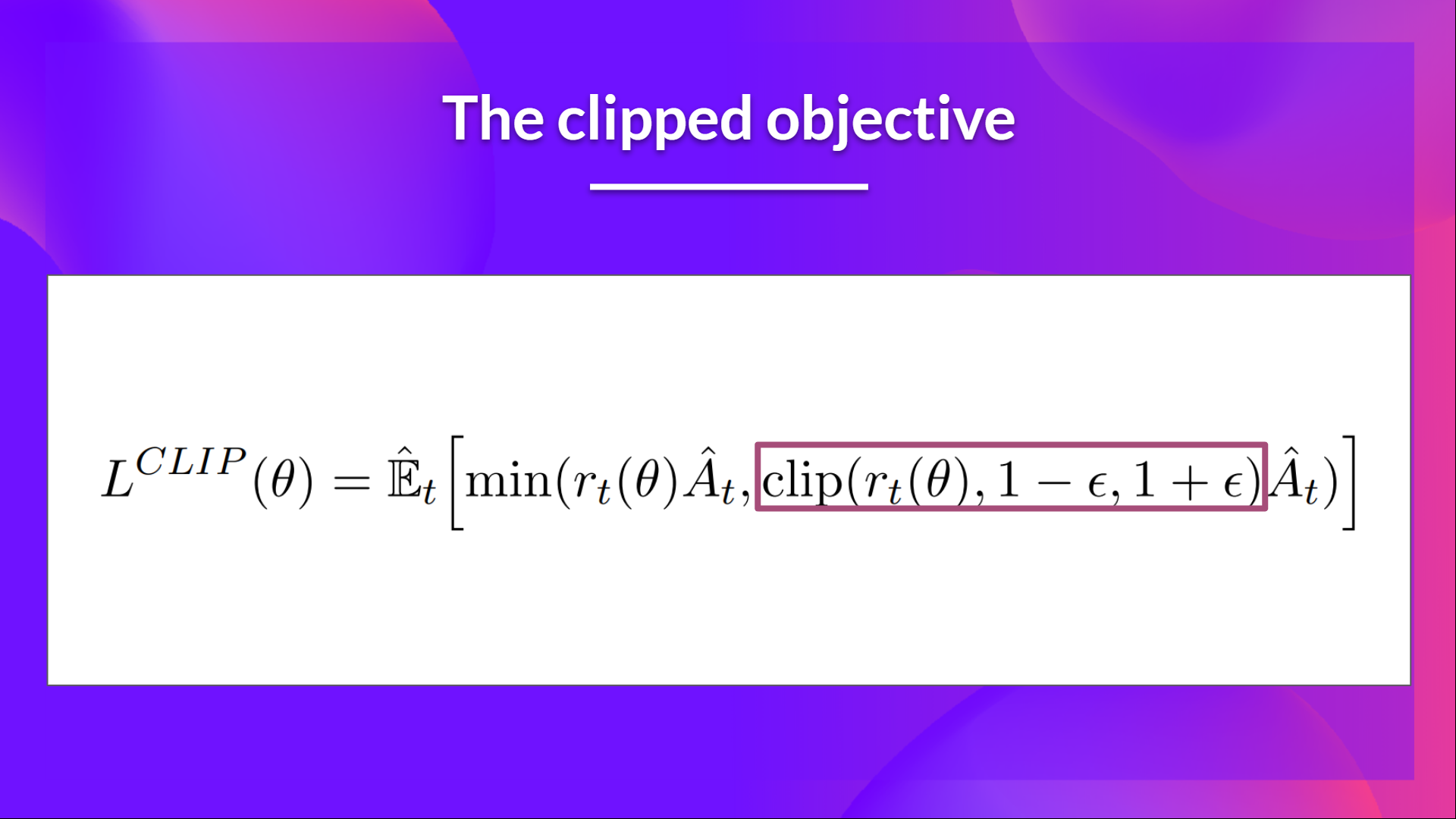
The Clipped Objective
-
If the ratio $r_t(\theta)$ deviates too much from 1, it indicates a significant change in the policy.
-
To prevent this, we clip the ratio: we ensure that we do not have a too large policy update.
-
Two solutions:
- TRPO: Trust Region Policy Optimization $\rightarrow$ constrains the policy update using a KL-divergence constraint. Complicated to implement.
- PPO: Proximal Policy Optimization $\rightarrow$ simpler to implement and computationally efficient. We use Clipped surrogate Objective function.
-
The clipped objective limits the change in the policy by clipping the ratio $r_t(\theta)$ to the range $[1 - \epsilon, 1 + \epsilon]$.
-
This prevents the policy from changing too much in a single update, leading to more stable learning.

-
Case 1 & 2, the clipping does not affect the objective because the ratio is within the clipping range.
-
Case 3 & 4, the ratio is below the clipping range $1 - \epsilon$.
- Case 3: if the advantage is positive, we want to increase the probability of taking that action, we still update the policy and do not clip it.
- Case 4: if the advantage is negative, we don’t want to decrease the probability of taking that action too much, so we clip the ratio to $1 - \epsilon$. The gradient will be zero in this case and we won’t update the policy for that action.
-
Case 5 & 6, the ratio is above the clipping range $1 + \epsilon$.
- Case 5: if the advantage is positive, we don’t want to increase the probability of taking that action too much, so we clip the ratio to $1 + \epsilon$. The gradient will be zero in this case and we won’t update the policy for that action.
- Case 6: if the advantage is negative, we want to decrease the probability of taking that action, we still update the policy and do not clip it.
-
We only update the policy with the unclipped objective part. When the minimum is the clipped part, the gradient will be zero and we won’t update the policy for that action.
-
So update policy only if:
- The ratio is within the clipping range.
- The ratio is outside the clipping range but the advantage leads to getting closer to the range:
- Ratio < $1 - \epsilon$ and advantage > 0
- Ratio > $1 + \epsilon$ and advantage < 0
-
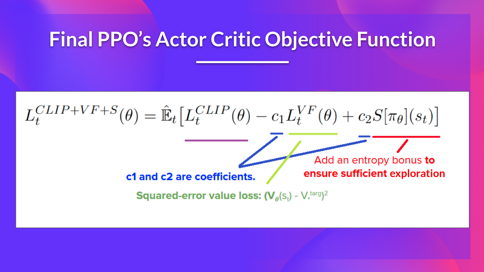
The final Clipped Surrogate Objective function for PPO Actor -Critic is: combination of Clipped Surrogate Objective, Value Loss Function, and Entropy Bonus.